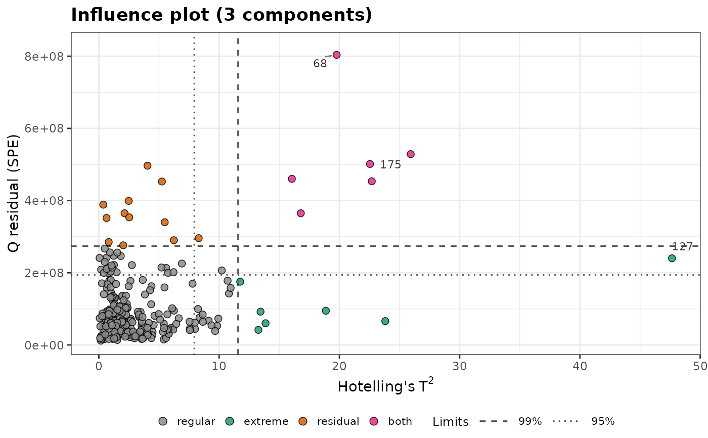
Hotelling's T-squared and Q Residuals of a PCA Model

Computes, for each sample, the two distances used to monitor a principal component analysis (PCA) model: Hotelling's $T^2$, the distance within the model plane of the first k components, and the Q residual (squared prediction error, SPE), the squared distance to that plane, with their limits at one or more confidence levels.

Usage

q_residuals(
  model,
  k,
  newdata = NULL,
  conf_level = 0.975,
  method = "jackson",
  t2_method = "f",
  center = TRUE,
  scale = FALSE
)

Arguments

model: A stats::prcomp() fit that kept all its components (the default of prcomp()), or a numeric matrix or data frame, on which a PCA is fitted with center and scale.
k: The number of components of the model.
newdata: Optional new samples (a matrix or data frame with the variables of the model), whose distances are computed instead of those of the calibration samples.
conf_level: The confidence level(s) of the limits: one or more values between 0 and 1. Default is 0.975.
method: The limit of Q: "jackson" (default, Jackson-Mudholkar) or "box".
t2_method: The distribution of the $T^2$ limit of the samples of the model: "f" (default) or "beta" (see hotelling_t2()).
center, scale: Passed to stats::prcomp() when model is data. Default is TRUE and FALSE.

Value

A tibble of class specproc_influence, with one row per sample: sample (row number), t2, its limits at each confidence level (in %, e.g. t2_limit_97.5), q, its limits (q_limit_97.5, ...) and outlier, the type of the sample at the highest confidence level: "regular", "extreme" (high $T^2$ only), "residual" (high Q only) or "both". Draw it with plot_influence().

Details

With scores $t_{ia}$ and eigenvalues $\lambda_a$, $$T^2_i = \sum_{a=1}^{k} \frac{t_{ia}^2}{\lambda_a}, \qquad Q_i = \lVert x_i - \hat{x}_i \rVert^2$$ where $\hat{x}_i$ is the reconstruction of the (centered and scaled) sample from the k components. A high $T^2$ is an extreme but well-modeled sample (for example, a high concentration); a high Q is a sample the model does not describe (another matrix, a contamination, an instrumental problem).

For the samples of the model, $T^2$ and its limits come from hotelling_t2() (F or Beta distribution, t2_method). For new samples, the limit is that of a new observation, $k(n+1)(n-1)/(n(n-k))\,F(k, n-k)$. The limit of Q is that of Jackson and Mudholkar (1979), from the eigenvalues of the components left out, or Box's (1954) scaled chi-square approximation (method = "box"); both tend to be slightly conservative. The Jackson-Mudholkar limit depends on a power $h_0$ of Q computed from these eigenvalues; when $h_0$ is close to zero (a few large eigenvalues followed by a long tail of small ones, common for spectra), its limit as $h_0 \to 0$, a lognormal approximation, is used. Samples are classified at the highest confidence level.

These are classical estimates, themselves affected by outliers: see robpca() and plot_outlier_map() for robust score and orthogonal distances. dmodx() gives the residual distance as a standard deviation, relative to that of the calibration samples.

References

Jackson, J.E., Mudholkar, G.S. (1979). Control procedures for residuals associated with principal component analysis. Technometrics, 21(3):341-349.
Box, G.E.P. (1954). Some theorems on quadratic forms applied in the study of analysis of variance problems, I. Annals of Mathematical Statistics, 25(2):290-302.
Nomikos, P., MacGregor, J.F. (1995). Multivariate SPC charts for monitoring batch processes. Technometrics, 37(1):41-59.

Author

Christian L. Goueguel

Examples

if (rlang::is_installed("HotellingEllipse", version = "1.3.0")) {
  data(forageLIBS)
  # the 380-430 nm window (Ca II H and K lines)
  wl <- suppressWarnings(as.numeric(names(forageLIBS)))
  spectra <- forageLIBS[which(wl > 380 & wl < 430)]
  pca <- stats::prcomp(spectra)
  influence <- q_residuals(pca, k = 3)
  influence[influence$outlier != "regular", ]
  plot_influence(influence, label = forageLIBS$Measurement)
  # several limits
  plot_influence(q_residuals(pca, k = 3, conf_level = c(0.95, 0.99)))
}