2. Preprocessing with recipe steps

Preprocessing turns raw spectra into variables ready for modeling. In specProc, each preprocessing method is also a recipes step (step_*()). A recipe is estimated on training data (prep()) and applied unchanged to new spectra (bake()), and within a tidymodels workflow it is re-estimated in every resample and can be tuned with the model. This vignette builds a recipe for the forage spectra, and uses it to predict potassium.

suppressPackageStartupMessages(library(mixOmics))
library(specProc)
library(recipes)
library(parsnip)
library(plsmod)
library(workflows)
library(tune)
library(rsample)
library(yardstick)
library(dplyr)
library(purrr)
library(ggplot2)
# mixOmics (the PLS engine) and MASS, which it attaches, have functions
# named like those of the tidyverse and tidymodels: use the latter
select <- dplyr::select
map <- purrr::map
tune <- tune::tune

data("forageLIBS")
spectra_id <- forageLIBS |> select(1:2) |> names()
minerals <- forageLIBS |> select(3:14) |> names()
spectra <- forageLIBS |> select(-all_of(c(spectra_id, minerals)))
wl <- as.numeric(names(spectra))

The recipe predicts K from the spectral channels. The identifiers and the other elements keep a role of their own, so they are carried along but not used as predictors:

base <- recipe(K ~ ., data = forageLIBS) |>
  update_role(all_of(spectra_id), all_of(setdiff(minerals, "K")), new_role = "id")

Baseline correction

The continuum emission of the plasma and the detector offset add a smooth background to every spectrum. step_baseline() removes it, by default with asymmetrically reweighted penalized least squares (baseline_arpls()). Its parameter lambda sets the stiffness of the baseline: too small, it cuts into the lines; too large, it misses the curvature of the continuum. baseline_arpls() shows the baseline itself:

region <- wl > 276 & wl < 290
fitted_baselines <- map(c(`1e3` = 1e3, `1e5` = 1e5, `1e7` = 1e7), \(lambda) {
  unlist(baseline_arpls(spectra[1, ], lambda = lambda, max.iter = 20)$background)[region]
})
first_spectrum <- tibble(wavelength = wl[region], counts = unlist(spectra[1, region]))

tibble(wavelength = wl[region], !!!fitted_baselines) |>
  tidyr::pivot_longer(-wavelength, names_to = "lambda", values_to = "counts") |>
  ggplot(aes(wavelength, counts)) +
  geom_line(data = first_spectrum, colour = "grey55") +
  geom_line(aes(colour = lambda), linewidth = 0.8) +
  coord_cartesian(ylim = c(800, 2500)) +
  labs(x = "Wavelength (nm)", y = "Counts (lines truncated)") +
  theme_bw() +
  theme(legend.position = "top")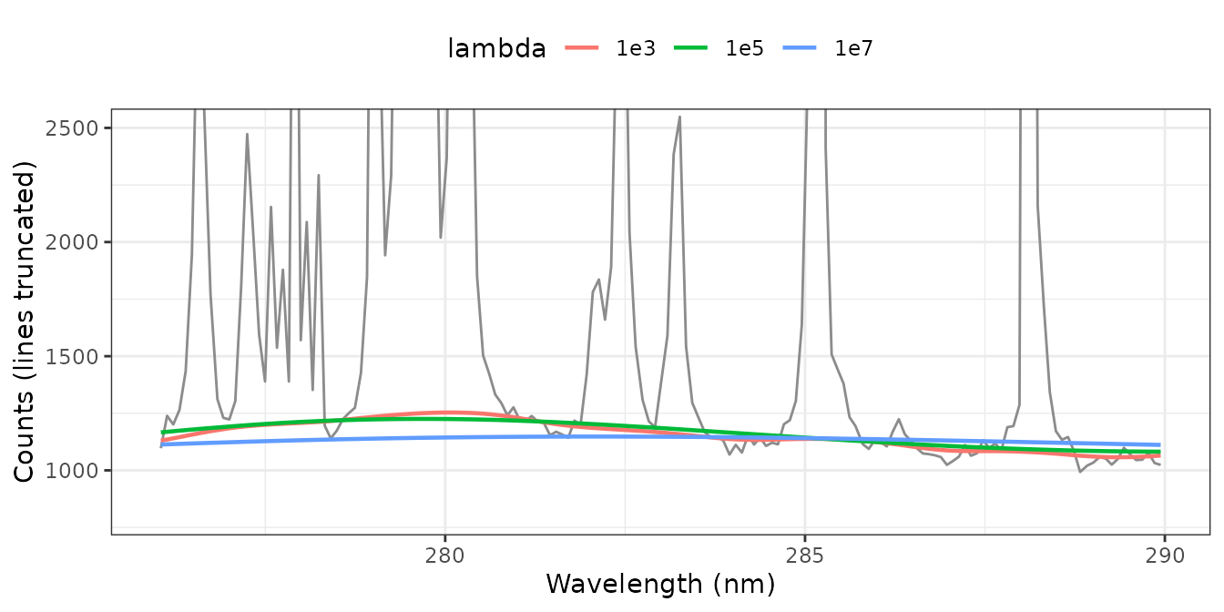

With lambda = 1e7, the baseline is too stiff to follow the broad hump of the continuum under the Mg lines near 280 nm; with 1e3, it starts to rise into the lines. 1e5 follows the continuum without touching them. lambda can also be tuned with the model (lambda = tune(), with the range of baseline_lambda()).

corrected <- base |>
  step_baseline(all_predictors(), lambda = 1e5, options = list(max.iter = 20))

step_baseline() corrects each spectrum on its own and estimates nothing from the training data, so it gives the same result inside or outside a resampling loop. To avoid repeating it in every recipe and every resample below, we apply it once and start the following recipes from the corrected spectra:

corrected_data <- corrected |> prep() |> bake(new_data = NULL)
base_corrected <- recipe(K ~ ., data = corrected_data) |>
  update_role(all_of(spectra_id), all_of(setdiff(minerals, "K")), new_role = "id")

Normalization

The intensity of every line changes from spectrum to spectrum with the ablated mass and the plasma conditions. Normalization divides each spectrum by a quantity that follows these changes:

Step	Divides each spectrum by
step_spectral_norm()	its total area, or its L1, L2 or maximum norm
step_snv()	its standard deviation, after centering (standard normal variate)
step_msc()	a regression on the mean spectrum (multiplicative scatter correction)
step_emsc()	an extended model with a polynomial baseline
step_line_ratio()	the intensity of a reference line (internal standard)

A good normalization brings the line intensities closer to the concentrations. step_line_intensities() replaces the channels by the intensities of chosen lines, so we compare the normalizations by the correlation of each line with the laboratory concentration of its element:

lines <- c(K = 769.896, Mg = 285.213, Ca = 317.933, Na = 589.592, Mn = 257.610, Fe = 259.940)
normalizations <- list(
  none = identity,
  area = \(r) step_spectral_norm(r, all_predictors(), method = "area"),
  SNV = \(r) step_snv(r, all_predictors()),
  MSC = \(r) step_msc(r, all_predictors()),
  `C I 247.86` = \(r) step_line_ratio(r, all_predictors(), reference = 247.856, window = 0.15)
)

imap(normalizations, \(normalize, name) {
  intensities <- base_corrected |>
    normalize() |>
    step_line_intensities(all_predictors(), lines = lines) |>
    prep() |>
    bake(new_data = NULL)
  map_dbl(names(lines), \(e) cor(intensities[[paste0("line_", e)]], forageLIBS[[e]],
                                 use = "complete.obs")) |>
    set_names(names(lines))
}) |>
  bind_rows(.id = "normalization") |>
  mutate(across(-normalization, \(r) round(r, 2)))
#> # A tibble: 5 × 7
#>   normalization     K    Mg    Ca    Na    Mn    Fe
#>   <chr>         <dbl> <dbl> <dbl> <dbl> <dbl> <dbl>
#> 1 none           0.54  0.42  0.5   0.76  0.7   0.92
#> 2 area           0.55  0.55  0.73  0.81  0.75  0.91
#> 3 SNV            0.63  0.48  0.65  0.8   0.75  0.92
#> 4 MSC            0.63  0.46  0.63  0.8   0.75  0.92
#> 5 C I 247.86     0.76  0.66  0.75  0.8   0.75  0.92

Normalizing to the carbon line C I 247.86 nm gives the highest correlations for K, Mg and Ca. Carbon is the main element of the organic matrix, and its content varies little between forages: it is an internal standard. The other normalizations help less. The correlations of Na, Mn and Fe change little: their concentrations vary over a much wider range than the normalization factor.

Other steps

Purpose	Steps
Smoothing, derivatives	step_savgol(), step_gap_derivative() (gap-segment derivative)
Compression	step_bin_spectra() (means of adjacent channels), step_wavelet() (wavelet coefficients), step_line_intensities() (line intensities)
Scaling	step_pareto_scale(), step_poisson_scale()
Removing unwanted variation	step_epo(), step_glsw(), step_osc(), step_direct_osc(), step_projected_osc(), step_opls(), step_o2pls(), step_y_gradient_glsw()
Robust transformations, PCA and PLS	step_robust_bcyj(), step_robpca(), step_rospca(), step_macropca(), step_cellpca(), step_rsimpls()
Replicate shots	step_reject_shots()

For example, step_wavelet() keeps the approximation coefficients of a discrete wavelet transform, a smoothed spectrum with 8 times fewer values at level = 3:

base_corrected |>
  step_wavelet(all_predictors(), level = 3) |>
  prep() |>
  bake(new_data = NULL) |>
  select(starts_with("wav_")) |>
  ncol()
#> [1] 894

Steps that use the outcome, such as step_opls() or step_osc(), must be estimated on training data only. Within a workflow, this is automatic.

A model for potassium

We keep 20% of the samples for testing. The data hold a few repeated samples, so the splits keep the spectra of a sample together:

set.seed(1)
split <- group_initial_split(corrected_data, group = Sample, prop = 0.8)
training_set <- training(split)
folds <- group_vfold_cv(training_set, group = Sample, v = 5)

The model is a partial least squares (PLS) regression, from the mixOmics engine of parsnip, with its number of components tuned. We compare three recipes: baseline correction followed by SNV, by the carbon internal standard, or by the carbon standard and a wavelet compression:

carbon_step <- \(r) step_line_ratio(r, all_predictors(), reference = 247.856, window = 0.15)

recipes <- list(
  SNV = base_corrected |> step_snv(all_predictors()),
  carbon = base_corrected |> carbon_step(),
  `carbon + wavelet` = base_corrected |> carbon_step() |>
    step_wavelet(all_predictors(), level = 3)
)

# mixOmics scales every predictor by default; scale = FALSE only centers
pls_model <- pls(num_comp = tune()) |>
  set_mode("regression") |>
  set_engine("mixOmics", scale = FALSE)

tuned <- map(recipes, \(rec) {
  tune_grid(workflow(rec, pls_model), resamples = folds,
            grid = tibble(num_comp = c(2, 4, 6, 8, 10, 12, 15)),
            metrics = metric_set(rmse, rsq))
})

map(tuned, \(res) show_best(res, metric = "rmse", n = 1)) |>
  bind_rows(.id = "recipe") |>
  select(recipe, num_comp, rmse = mean, std_err)
#> # A tibble: 3 × 4
#>   recipe           num_comp  rmse std_err
#>   <chr>               <dbl> <dbl>   <dbl>
#> 1 SNV                     8 0.262  0.0187
#> 2 carbon                 10 0.257  0.0183
#> 3 carbon + wavelet       12 0.256  0.0224

map(tuned, collect_metrics) |>
  bind_rows(.id = "recipe") |>
  filter(.metric == "rmse") |>
  ggplot(aes(num_comp, mean, colour = recipe)) +
  geom_line() +
  geom_point() +
  labs(x = "PLS components", y = "Cross-validated RMSE (% K)", colour = NULL) +
  theme_bw()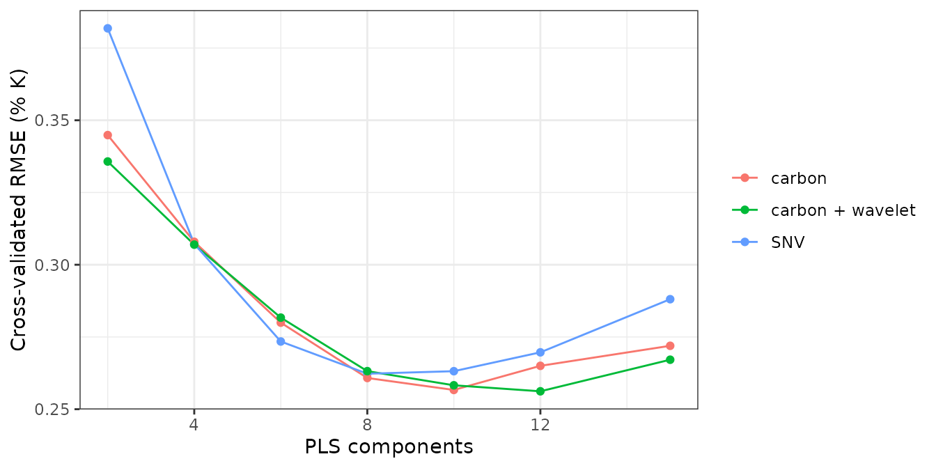

The three recipes give similar errors once the number of components is tuned: PLS finds the potassium information in all of them, and the normalization matters less for a multivariate model than for a single line. The carbon + wavelet recipe is the best by a small margin. We refit it on the whole training set with its best number of components, and evaluate it once on the test samples:

final <- workflow(recipes[[best_recipe]], pls_model) |>
  finalize_workflow(select_best(tuned[[best_recipe]], metric = "rmse")) |>
  last_fit(split, metrics = metric_set(rmse, rsq))
collect_metrics(final)
#> # A tibble: 2 × 4
#>   .metric .estimator .estimate .config        
#>   <chr>   <chr>          <dbl> <chr>          
#> 1 rmse    standard       0.321 pre0_mod0_post0
#> 2 rsq     standard       0.694 pre0_mod0_post0

The test error, 0.32% K, is somewhat larger than the cross-validated one (0.26%): with 74 test spectra, it is itself uncertain.

collect_predictions(final) |>
  ggplot(aes(K, .pred)) +
  geom_abline(colour = "grey50", linetype = "dashed") +
  geom_point(alpha = 0.6) +
  coord_equal() +
  labs(x = "Laboratory K (%)", y = "Predicted K (%)") +
  theme_bw()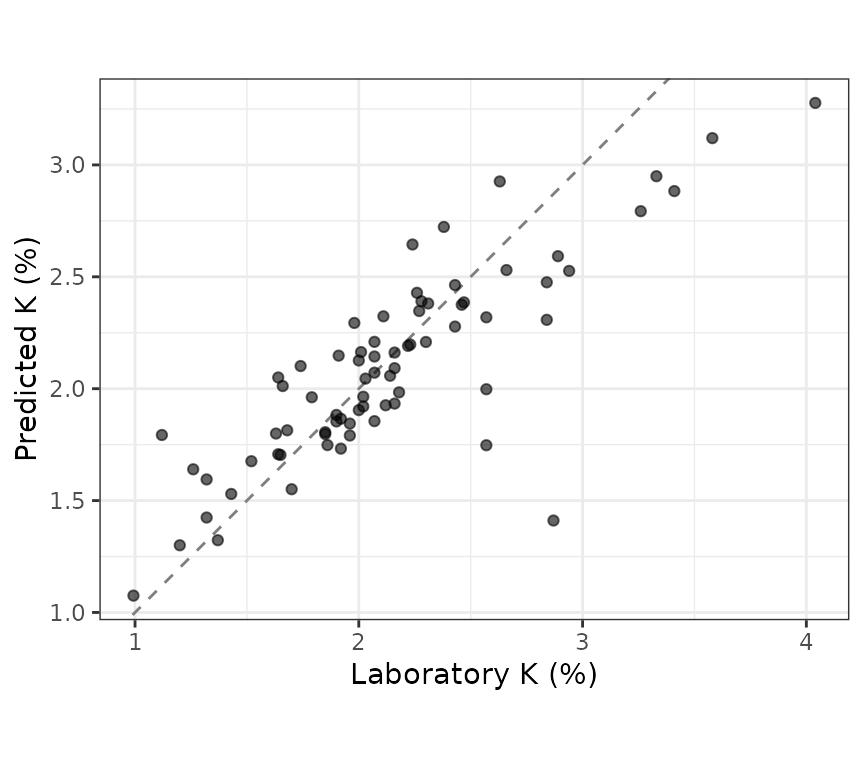

The fitted workflow applies every step, with the values estimated on the training data, to new spectra: predict(extract_workflow(final), new_data). The prepped recipe also shows what each step estimated, with tidy(). The next vignette, vignette("calibration"), builds univariate calibration curves and computes the figures of merit of both kinds of models.