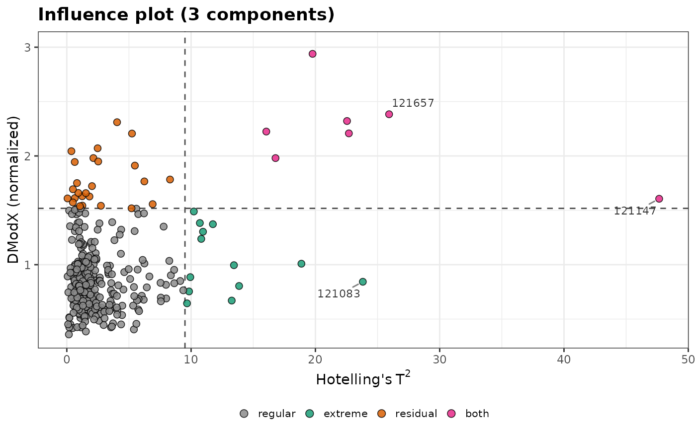
Distance to the Model (DModX) of a PCA Model

Computes the distance of each sample to a principal component analysis (PCA) model in the space of the variables (DModX): the residual standard deviation of the sample, normalized by that of the calibration samples, with its limits at one or more confidence levels, and Hotelling's $T^2$ for the influence plot.

Usage

dmodx(
  model,
  k,
  newdata = NULL,
  conf_level = 0.975,
  normalized = TRUE,
  df = "effective",
  t2_method = "f",
  center = TRUE,
  scale = FALSE
)

Arguments

model: A stats::prcomp() fit that kept all its components (the default of prcomp()), or a numeric matrix or data frame, on which a PCA is fitted with center and scale.
k: The number of components of the model.
newdata: Optional new samples (a matrix or data frame with the variables of the model), whose distances are computed instead of those of the calibration samples.
conf_level: The confidence level(s) of the limits: one or more values between 0 and 1. Default is 0.975.
normalized: A logical: DModX relative to the residual standard deviation of the calibration samples (TRUE, default), or absolute.
df: The degrees of freedom of the limit: "effective" (default) or "nominal" (see details).
t2_method: The distribution of the $T^2$ limit of the samples of the model: "f" (default) or "beta" (see hotelling_t2()).
center, scale: Passed to stats::prcomp() when model is data. Default is TRUE and FALSE.

Value

A tibble of class specproc_influence, with one row per sample: sample, t2 and its limits (as for q_residuals()), dmodx, its limits at each confidence level (dmodx_limit_97.5, ...), and outlier, the type of the sample at the highest confidence level. Draw it with plot_influence().

Details

With the residuals $e_{ij}$ of the $K$ variables after k components, for $N$ calibration samples (and $A_0 = 1$ if the data are centered), $$s_i = \sqrt{\frac{\sum_j e_{ij}^2}{K - k}}\,\sqrt{\frac{N}{N - k - A_0}}, \qquad s_0 = \sqrt{\frac{\sum_i \sum_j e_{ij}^2}{(N - k - A_0)(K - k)}}$$ (the correction factor $\sqrt{N / (N - k - A_0)}$ applies to the calibration samples only). DModX is $s_i / s_0$ (normalized, default) or $s_i$. Its squared ratio follows an F distribution with $\nu$ and $(N - k - A_0)\nu$ degrees of freedom, so the limit of the normalized DModX is $\sqrt{F_{1-\alpha}}$ (times $s_0$ for the absolute DModX).

The nominal degrees of freedom are $\nu = K - k$ (df = "nominal"), as if the residuals of the variables were independent. For spectra, with far more (correlated) channels than samples, this gives a limit close to 1 that flags a large share of ordinary samples. With df = "effective" (default), $\nu$ is the effective number of residual dimensions, $\theta_1^2 / \theta_2$ from the eigenvalues $\lambda_a$ of the components left out ($\theta_j = \sum_{a > k} \lambda_a^j$, as in Box's approximation of Q), which is $K - k$ when the residuals are independent with equal variances. DModX is then consistent with the Q residuals of q_residuals(), of which it is a scaled square root.

References

Eriksson, L., Johansson, E., Kettaneh-Wold, N., Trygg, J., Wikström, C., Wold, S. (2006). Multi- and Megavariate Data Analysis, Part I, 2nd ed. Umetrics Academy, Umeå.
Box, G.E.P. (1954). Some theorems on quadratic forms applied in the study of analysis of variance problems, I. Annals of Mathematical Statistics, 25(2):290-302.

Author

Christian L. Goueguel

Examples

if (rlang::is_installed("HotellingEllipse", version = "1.3.0")) {
  data(forageLIBS)
  # the 380-430 nm window (Ca II H and K lines)
  wl <- suppressWarnings(as.numeric(names(forageLIBS)))
  spectra <- forageLIBS[which(wl > 380 & wl < 430)]
  pca <- stats::prcomp(spectra)
  d <- dmodx(pca, k = 3)
  d[d$outlier != "regular", ]
  plot_influence(d, label = forageLIBS$Measurement)
}