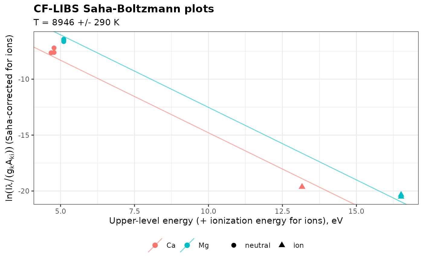
Calibration-Free LIBS Quantification

Estimates the elemental composition of a sample from the intensities of its emission lines, without calibration standards, by the calibration-free LIBS (CF-LIBS) method of Ciucci et al. (1999).

Usage

cf_libs(
  lines,
  electron_density = NULL,
  temperature = NULL,
  method = NULL,
  partition = NULL,
  ionization_energy = NULL,
  reference = NULL,
  units = "energy",
  timeout = 120
)

Arguments

lines: A data frame with one row per line and columns species (such as "Ca I" or "Ca II"; stages I and II), intensity (integrated line intensity), wavelength (nm), Aki (s$^{-1}$), gk and Ek (eV), such as the lines of nist_lines() with measured intensities.
electron_density: The electron density, in cm$^{-3}$. Needed for the elements observed in one ionization stage only; without it, only the observed stage of these elements is counted, with a warning.
temperature: The plasma temperature, in K. By default, it is estimated from the lines.
method: "boltzmann" or "saha-boltzmann" (see details). By default, "saha-boltzmann" when electron_density is given, "boltzmann" otherwise.
partition: The partition functions: NULL (default) to compute them from the levels of the NIST Atomic Spectra Database (see nist_levels(); needs an internet connection), a data frame of levels with columns species, g and energy (eV), or a function of the species and the temperature returning the partition functions.
ionization_energy: The ionization energies of the neutral atoms, in eV, named by element (c(Ca = 6.113)) or neutral species (c("Ca I" = 6.113)): for all elements with the Saha-Boltzmann method, and otherwise for the elements observed in one stage only and to truncate the partition functions computed from levels. By default, they are taken from the NIST database (see nist_ionization_energy()).
reference: An optional known mass fraction of one element, named by the element, such as c(Ca = 0.35), used instead of closure.
units: The units of intensity: "energy" (default) or "photons", as in boltzmann().
timeout: The timeout of the NIST downloads, in seconds. Default is 120.

Value

An object of class specproc_cflibs, a list with

composition: a tibble with, for each element, the atomic_fraction and mass_fraction, and the stages observed (a stage computed by the Saha equation is noted "Saha");
species: a tibble with, for each species, the number of lines, the intercept of its own Boltzmann plot, its partition function, its relative number density and whether it was observed;
temperature, temperature_se (K) and electron_density;
points: the points of the plots (for the Saha-Boltzmann method, the abscissa of ions includes the ionization energy and the ordinate the Saha correction), intercept, the intercept of each plot, and fit, the lm fit;
method and the number of iterations of the Saha-Boltzmann fit.

Use plot_boltzmann() to draw the Boltzmann plots.

Details

In a plasma in local thermodynamic equilibrium (LTE), optically thin and of the same composition as the sample, the intensity of a line of species $s$ satisfies $$\ln\frac{I\lambda}{g_k A_{ki}} = -\frac{E_k}{k_B T} + \ln\frac{F C_s}{U_s(T)}$$ where $C_s$ is the concentration of the species, $U_s(T)$ its partition function and $F$ an experimental factor common to all lines. The Boltzmann plots of all species are therefore parallel lines:

The temperature is estimated from their common slope, by a least-squares fit with one intercept per plot (unless temperature is given).
The relative number density of each species follows from the intercept $q_s$ of its plot, $F C_s = U_s(T) e^{q_s}$.
The density of an ionization stage that is not observed is computed with the Saha equation, from the electron density (see electron_density()) and the ionization energy.
The factor $F$ is eliminated by closure (the concentrations of the elements sum to 1), or, with reference, by the known mass fraction of one element (internal reference), which is useful when some elements of the sample are not measured.

Two methods place the lines on the plots:

"boltzmann" (Ciucci et al., 1999): one Boltzmann plot per species, with its own intercept. The temperature rests on the range of upper-level energies within each species, often narrow (1 to 2 eV), so it can be imprecise.
"saha-boltzmann" (the default when electron_density is given): one Saha-Boltzmann plot per element, on which the lines of the ion are placed with the Saha equation, as in saha_boltzmann(). The energy range is extended by the ionization energy, which gives a much more precise temperature, and the ionization balance of each element follows from the Saha equation. It needs the ionization energies of all elements.

At least one plot needs two lines or more of different upper-level energies.

When the partition functions are computed from energy levels, the levels of the neutral atoms above their ionization energy, lowered by the Debye-Hückel correction when electron_density is given, are left out (see partition_function()). This needs the ionization energies of all elements observed as neutral atoms.

The mass fractions are computed from the atomic fractions with the standard atomic weights. The result is only as good as its assumptions: all major elements must be measured (with closure), the lines must be optically thin (see self_absorption()), the intensities corrected for the spectral response of the instrument, and the atomic data accurate (prefer lines of accuracy B or better in nist_lines()).

References

Ciucci, A., Corsi, M., Palleschi, V., Rastelli, S., Salvetti, A., Tognoni, E. (1999). New procedure for quantitative elemental analysis by laser-induced plasma spectroscopy. Applied Spectroscopy, 53(8):960-964.
Tognoni, E., Cristoforetti, G., Legnaioli, S., Palleschi, V. (2010). Calibration-free laser-induced breakdown spectroscopy: state of the art. Spectrochimica Acta Part B, 65(1):1-14.

Author

Christian L. Goueguel

Examples

data(forageLIBS)
mean_spectrum <- colMeans(forageLIBS[-(1:14)])
# calcium and magnesium lines, with their atomic data from the NIST database
atomic <- data.frame(
  species = c("Ca I", "Ca I", "Ca I", "Ca II", "Ca II", "Mg I", "Mg I", "Mg I", "Mg II", "Mg II"),
  wavelength = c(428.301, 430.253, 445.478, 315.887, 317.933,
                 516.732, 517.268, 518.360, 279.078, 279.800),
  Aki = c(4.34e7, 1.36e8, 8.70e7, 3.10e8, 3.60e8, 1.13e7, 3.37e7, 5.61e7, 4.01e8, 4.79e8),
  gk = c(5, 5, 7, 4, 6, 3, 3, 3, 4, 6),
  Ek = c(4.780, 4.780, 4.681, 7.047, 7.050, 5.108, 5.108, 5.108, 8.864, 8.864)
)
# partition functions, interpolated from a table (see partition_function())
partition <- function(species, temperature) {
  grid <- c(6000, 8000, 10000, 12000)
  table <- rbind(`Ca I` = c(1.407, 2.401, 4.499, 8.356), `Ca II` = c(2.389, 2.917, 3.560, 4.262),
                 `Mg I` = c(1.049, 1.207, 1.597, 2.463), `Mg II` = c(2.001, 2.010, 2.036, 2.087))
  vapply(species, function(s) exp(stats::approx(grid, log(table[s, ]), xout = temperature)$y),
         numeric(1))
}
fit <- cf_libs(line_intensities(mean_spectrum, atomic, baseline = TRUE),
               electron_density = 1.9e17, partition = partition,
               ionization_energy = c(Ca = 6.113, Mg = 7.646))
fit
#> Calibration-free LIBS (10 lines, 4 species; Saha-Boltzmann plots)
#> 
#> Temperature:  8946 +/- 290 K
#> Ne:           1.9e+17 cm-3
#> Normalization: closure
#> 
#>  element atomic_fraction mass_fraction stages
#>  Ca      0.4512          0.5755        I, II 
#>  Mg      0.5488          0.4245        I, II 
plot_boltzmann(fit)