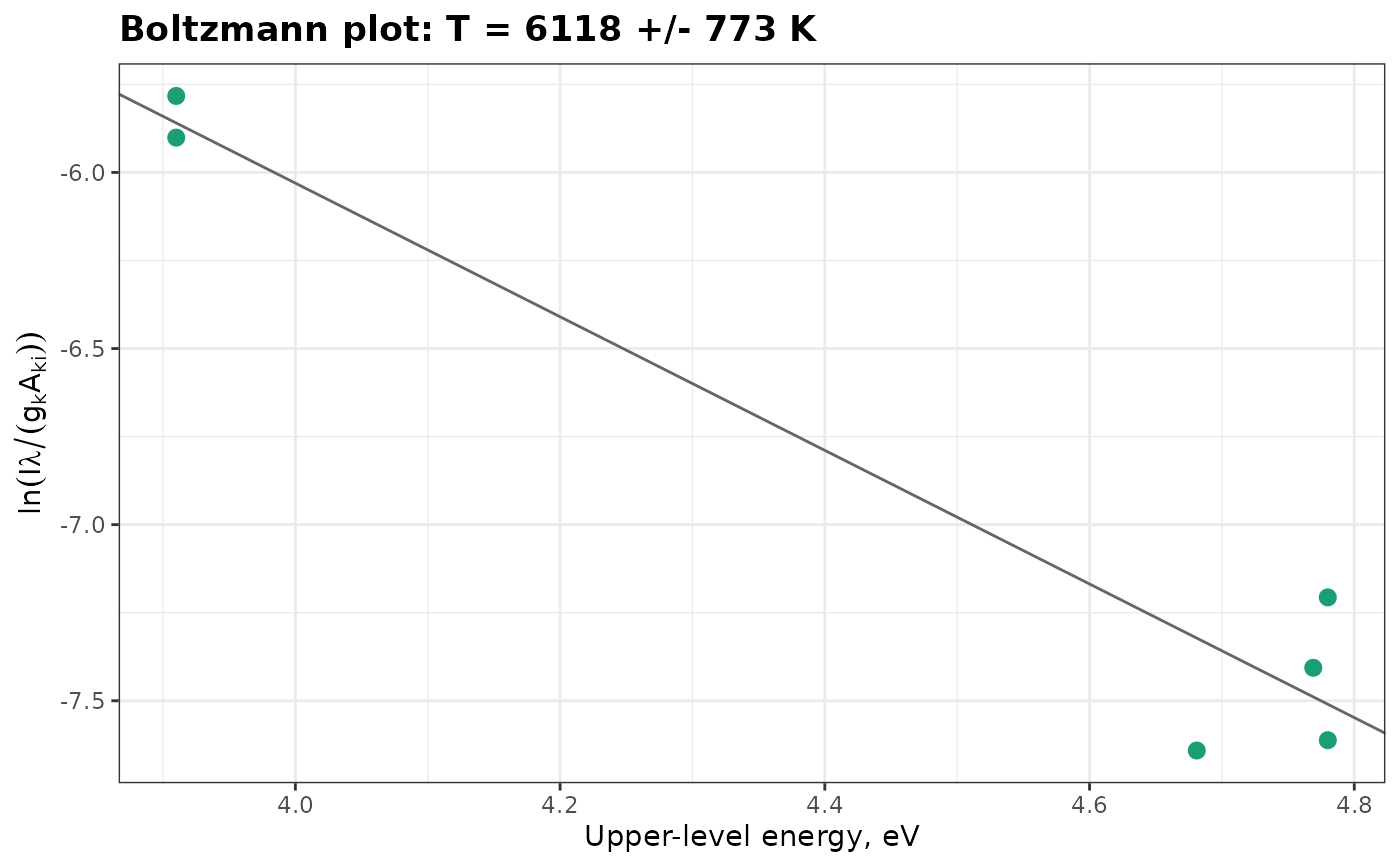
Plasma Temperature from a Boltzmann Plot

Estimates the excitation temperature of a plasma in local thermodynamic equilibrium (LTE) from the intensities of several lines of the same species, by a Boltzmann plot.

Usage

boltzmann(lines, units = "energy")

Arguments

lines: A data frame with one row per line and columns intensity (integrated line intensity), wavelength (nm), Aki (transition probability, s$^{-1}$), gk (upper-level degeneracy) and Ek (upper-level energy, eV).
units: The units of intensity: "energy" (default; radiance or energy-calibrated counts) or "photons" (photon counts).

Value

An object of class specproc_boltzmann, a list with

temperature and temperature_se: the temperature and its standard error, in K;
r_squared: the coefficient of determination of the fit;
points: a tibble with the abscissa x (eV) and ordinate y of each line;
fit: the lm fit of y on x.

Use plot_boltzmann() to draw the plot.

Details

In LTE, the integrated intensity of a line emitted from an upper level of energy $E_k$ and degeneracy $g_k$, with transition probability $A_{ki}$ and wavelength $\lambda$, satisfies $$\ln\frac{I\lambda}{g_k A_{ki}} = -\frac{E_k}{k_B T} + C$$ for intensities in energy units, or $\ln(I / g_k A_{ki})$ for photon counts (units = "photons"). A least-squares line through the points gives the temperature from its slope, $T = -1/(k_B\,\mathrm{slope})$, and its standard error from that of the slope.

The intensities must be corrected for the spectral response of the instrument, and the lines must be optically thin (see self_absorption()). A wide range of upper-level energies gives a more precise temperature. Atomic data ($A_{ki}$, $g_k$, $E_k$) can be taken from the NIST Atomic Spectra Database (https://physics.nist.gov/PhysRefData/ASD/lines_form.html).

References

Cristoforetti, G., De Giacomo, A., Dell'Aglio, M., Legnaioli, S., Tognoni, E., Palleschi, V., Omenetto, N. (2010). Local thermodynamic equilibrium in laser-induced breakdown spectroscopy: beyond the McWhirter criterion. Spectrochimica Acta Part B, 65(1):86-95.

Author

Christian L. Goueguel

Examples

data(forageLIBS)
mean_spectrum <- colMeans(forageLIBS[-(1:14)])
# calcium lines, with their atomic data from the NIST database
atomic <- data.frame(
  species = c(rep("Ca I", 6), rep("Ca II", 4)),
  stage = c(rep(1, 6), rep(2, 4)),
  wavelength = c(428.301, 430.253, 431.865, 445.478, 612.222, 616.217,
                 315.887, 317.933, 370.603, 373.690),
  Aki = c(4.34e7, 1.36e8, 7.40e7, 8.70e7, 2.87e7, 4.77e7, 3.10e8, 3.60e8, 8.80e7, 1.70e8),
  gk = c(5, 5, 3, 7, 3, 3, 4, 6, 2, 2),
  Ek = c(4.780, 4.780, 4.769, 4.681, 3.910, 3.910, 7.047, 7.050, 6.468, 6.468)
)
lines <- line_intensities(mean_spectrum, atomic, baseline = TRUE)
fit <- boltzmann(lines[lines$stage == 1, ])
fit
#> Boltzmann plot (6 lines)
#> 
#> Temperature:  6118 +/- 773 K
#> R-squared:    0.94
plot_boltzmann(fit)