
lwpls implements locally-weighted partial least squares (LW-PLS) for the tidymodels ecosystem.
LW-PLS is a just-in-time learning method used in chemometrics and process monitoring (soft sensors). Instead of fitting a single global model, it builds a dedicated weighted PLS model around each new sample, where every training sample is weighted by its similarity to that sample. A linear method can therefore capture nonlinear and time-varying relationships.
Features
-
lwpls(): a parsnip model for regression (one or more outcomes) and classification (LW-PLS-DA). - Two similarity indexes: the Euclidean distance of the original LW-PLS, and the covariance-based index of CbLW-PLS (
similarity = "covariance"). -
Robust local models, by partial robust M-regression (
set_engine("lwpls", robust = TRUE)), and sparse local models that select their own predictors (sparsity), with thetrimmed_rmse()metric to tune robust models on contaminated data. - A native implementation, validated against Kaneko’s reference implementation, with the prediction kernel written in C++ (RcppArmadillo). Queries are processed in blocks, so most of the work runs as BLAS matrix-matrix products.
- Tuning with tune and dials:
localization()andsimilarity()are tuning parameters, and all values ofnum_compare evaluated from a single fit (the “submodel trick”). -
lwpls_fit(): a standalone hardhat modeling function with matrix, data frame, formula and recipe interfaces. -
Diagnostics for spectroscopy (
lwpls_local()) with publication-ready ggplot2 plots: reliability of each prediction (applicability domain), local regression vectors along the spectrum, robust weights that point to wrong reference values, and wavelengths selected by sparse models.
Installation
Install a prebuilt binary from r-universe, which needs no compiler:
install.packages(
  "lwpls",
  repos = c("https://christiangoueguel.r-universe.dev", "https://cloud.r-project.org")
)
Or build the development version from GitHub with:
# install.packages("pak")
pak::pak("ChristianGoueguel/lwpls")
Building from source compiles C++ code, so it needs the R compiler tools. On macOS, that includes gfortran from https://mac.r-project.org/tools/.
Example
Predict the water content of meat samples from their near-infrared spectra and tune both hyperparameters with cross-validation:
library(tidymodels)
library(lwpls)

data(meats, package = "modeldata")
meats <- meats |> select(-fat, -protein)
set.seed(123)
meats_split <- initial_split(meats, prop = 0.75)
meats_folds <- vfold_cv(training(meats_split), v = 5)

lwpls_wflow <- workflow(
  water ~ .,
  lwpls(
    num_comp = tune(),
    localization = tune()
  ) |>
    set_mode("regression")
)

lwpls_grid <- grid_regular(
  num_comp(c(1, 15)),
  localization(),
  levels = c(num_comp = 15, localization = 8)
)

lwpls_res <- tune_grid(lwpls_wflow, meats_folds, grid = lwpls_grid)
show_best(lwpls_res, metric = "rmse", n = 3)
#> # A tibble: 3 × 8
#>   num_comp localization .metric .estimator  mean     n std_err .config
#>      <int>        <dbl> <chr>   <chr>      <dbl> <int>   <dbl> <chr>
#> 1       10          0.5 rmse    standard    1.66     5   0.156 pre0_mod077_post0
#> 2       13          0.5 rmse    standard    1.68     5   0.198 pre0_mod101_post0
#> 3        9          0.5 rmse    standard    1.70     5   0.174 pre0_mod069_post0
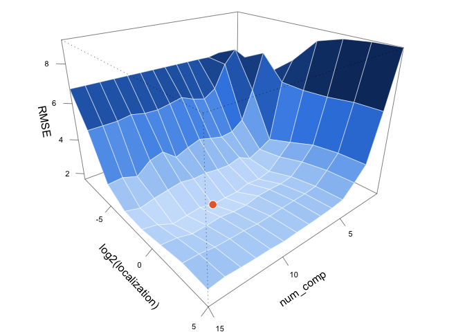
The 120 candidate models are evaluated with only 8 fits per resample. Their cross-validated RMSE forms a surface over the two hyperparameters, with a valley between very local models and global PLS (the best model is the orange point):
rmse_grid <- lwpls_res |>
  collect_metrics() |>
  filter(.metric == "rmse") |>
  select(num_comp, localization, rmse = mean)
best <- slice_min(rmse_grid, rmse)
# color each facet by its mean RMSE
rmse_mat <- with(rmse_grid, tapply(rmse, list(num_comp, log2(localization)), mean))
n <- dim(rmse_mat)
facets <- (rmse_mat[-1, -1] + rmse_mat[-1, -n[2]] + rmse_mat[-n[1], -1] + rmse_mat[-n[1], -n[2]]) / 4
blues <- colorRampPalette(c("#cde2fb", "#3987e5", "#0d366b"))(50)

par(mar = c(1, 0, 0, 0))
view <- persp(
  x = as.numeric(rownames(rmse_mat)),
  y = as.numeric(colnames(rmse_mat)),
  z = rmse_mat,
  theta = 140,
  phi = 25,
  expand = 0.7,
  ticktype = "detailed",
  col = blues[cut(facets, 50)],
  border = "white",
  lwd = 0.5,
  xlab = "num_comp",
  ylab = "log2(localization)",
  zlab = "RMSE", cex.axis = 0.7
)
points(
  trans3d(best$num_comp, log2(best$localization), best$rmse, view),
  pch = 21,
  bg = "#eb6834",
  col = "white",
  cex = 1.6
)
The final model is evaluated on the test set:
lwpls_wflow |>
  finalize_workflow(select_best(lwpls_res, metric = "rmse")) |>
  last_fit(meats_split) |>
  collect_metrics()
#> # A tibble: 2 × 4
#>   .metric .estimator .estimate .config
#>   <chr>   <chr>          <dbl> <chr>
#> 1 rmse    standard       1.38  pre0_mod0_post0
#> 2 rsq     standard       0.978 pre0_mod0_post0
Each prediction comes from its own local model. lwpls_local() returns these models with their diagnostics; for example, their regression vectors along the spectrum (100 channels between 850 and 1050 nm) show how the bands used change with the water content:
final_fit <- lwpls_wflow |>
  finalize_workflow(select_best(lwpls_res, metric = "rmse")) |>
  fit(training(meats_split))

final_fit |>
  lwpls_local(testing(meats_split), wavelength = seq(850, 1050, length.out = 100)) |>
  plot_coefficients(axis_label = "Wavelength (nm)")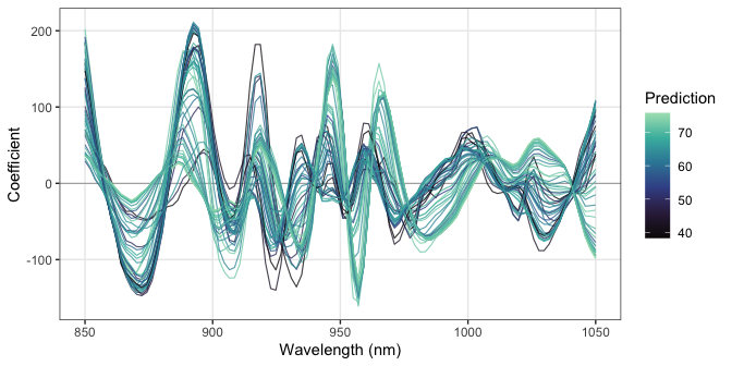
See vignette("lwpls") for more details, including the comparison with global PLS and classification, vignette("robust-sparse") for robust and sparse local models, and vignette("diagnostics") for the diagnostic plots.
How it works
For a query sample \(x_q\), each training sample \(x_i\) receives the weight
\[\omega_i = \exp\left(-\frac{\lVert x_i - x_q \rVert}{\sigma_d \varphi}\right)\]
where \(\sigma_d\) is the standard deviation of the distances and \(\varphi\) is the localization parameter. A PLS model with num_comp components is then fitted with these weights, and the query is projected onto it. Small values of \(\varphi\) give very local models; large values give global PLS.
References
- Kim, S., Kano, M., Nakagawa, H. and Hasebe, S. (2011). Estimation of active pharmaceutical ingredients content using locally weighted partial least squares and statistical wavelength selection. International Journal of Pharmaceutics, 421(2), 269–274. doi:10.1016/j.ijpharm.2011.10.007
- Bevilacqua, M. and Marini, F. (2014). Local classification: Locally weighted-partial least squares-discriminant analysis (LW-PLS-DA). Analytica Chimica Acta, 838, 20–30. doi:10.1016/j.aca.2014.05.057
- Hazama, K. and Kano, M. (2015). Covariance-based locally weighted partial least squares for high-performance adaptive modeling. Chemometrics and Intelligent Laboratory Systems, 146, 55–62. doi:10.1016/j.chemolab.2015.05.007
- Serneels, S., Croux, C., Filzmoser, P. and Van Espen, P. J. (2005). Partial robust M-regression. Chemometrics and Intelligent Laboratory Systems, 79(1–2), 55–64. doi:10.1016/j.chemolab.2005.04.007
- Hoffmann, I., Serneels, S., Filzmoser, P. and Croux, C. (2015). Sparse partial robust M regression. Chemometrics and Intelligent Laboratory Systems, 149, 50–59. doi:10.1016/j.chemolab.2015.09.019
- Lesnoff, M., Metz, M. and Roger, J.-M. (2020). Comparison of locally weighted PLS strategies for regression and discrimination on agronomic NIR data. Journal of Chemometrics, 34(5), e3209. doi:10.1002/cem.3209