Plots of LW-PLS local models — lwpls

Publication-ready plots of the local models returned by lwpls_local():

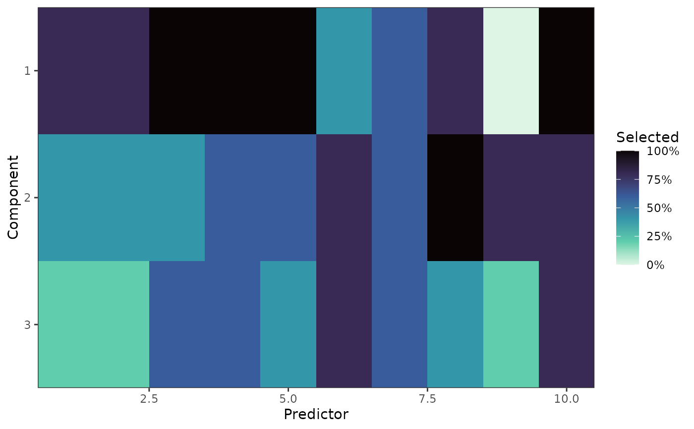
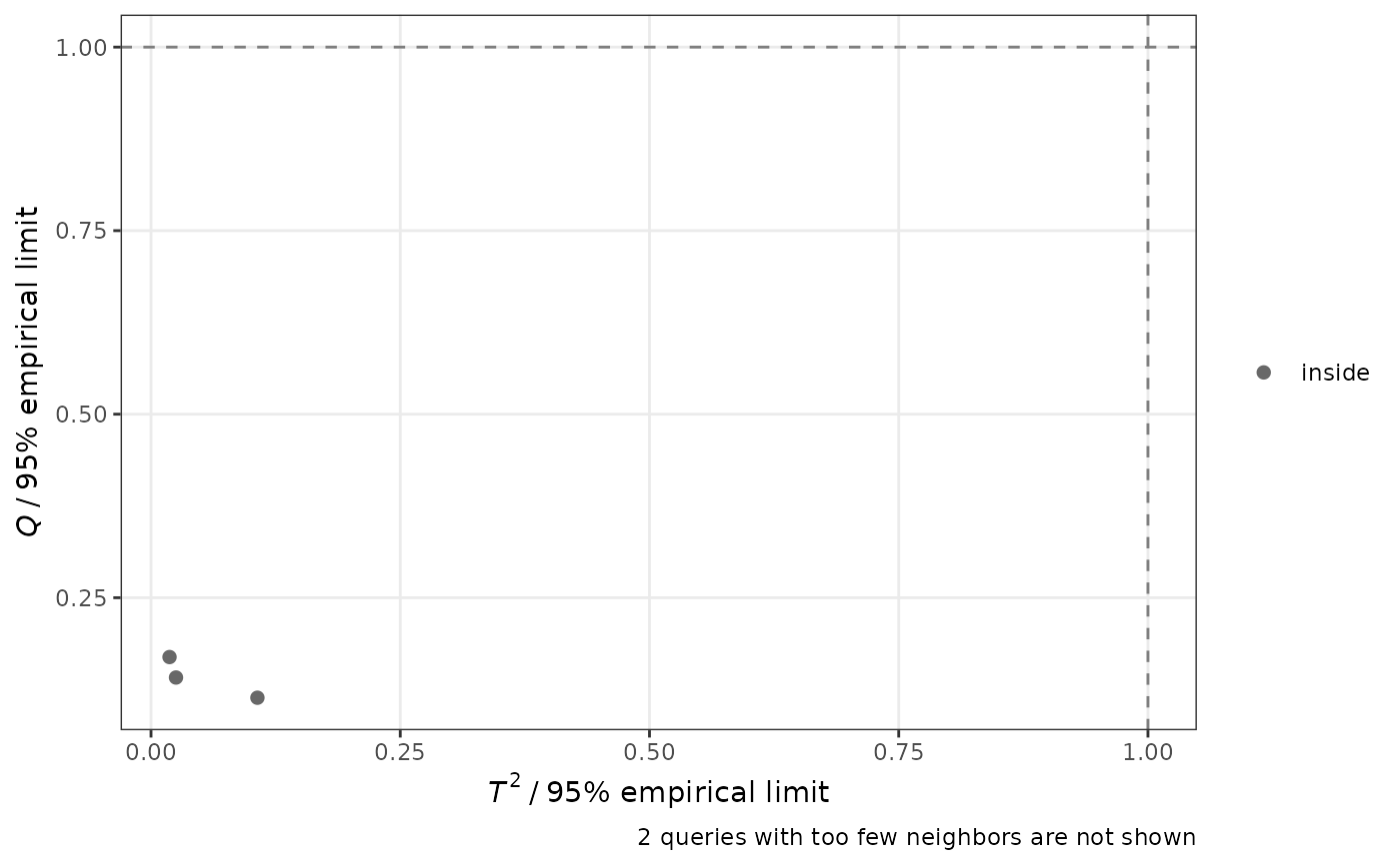
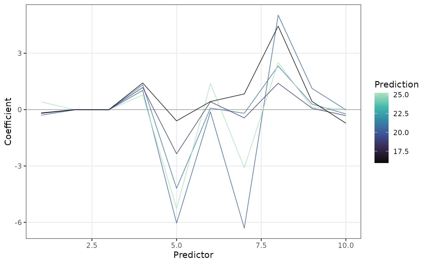
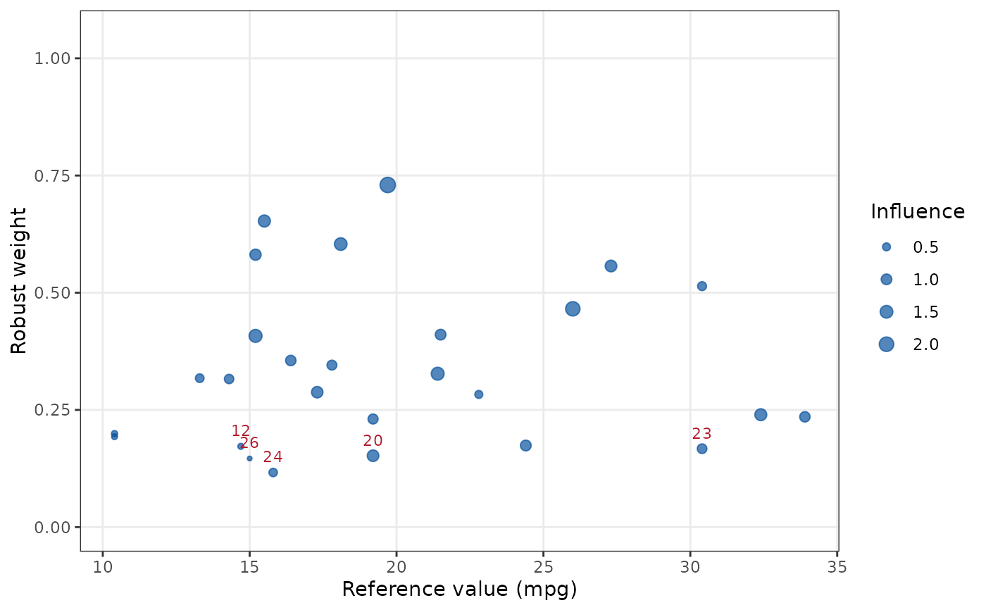
plot_reliability(): the \(T^2\) and \(Q\) statistics of the queries divided by their theoretical or empirical limits, or their percentile ranks among the training samples of their local models (see lwpls_local()). Queries beyond a limit are extrapolations of their local model, and their predictions should be checked.
plot_coefficients(): the regression coefficients (or VIP) of the local models along the spectral axis, as one line per query colored by its prediction, or as a heatmap of the queries ordered by their prediction. They show which bands drive the predictions and how they change across the range of the outcome.
plot_robust_weights(): the robust weights of the training samples (robust models), averaged over the local models in which they take part. Samples with low weights, often wrong reference values, are labeled.
plot_selection(): how often each predictor is selected by the sparse local models (sparse models): for each component (default), or by the local models as a whole (any component), with the mean spectrum for reference. On smooth spectra, the components of a sparse model often select different bands, so that almost all predictors are used by the model as a whole: the selection per component is then more informative.

All plots are ggplot2 objects that can be modified further.

Usage

plot_reliability(object, reference = NULL, labels = 5, log = FALSE, ...)

plot_coefficients(
  object,
  type = c("coefficients", "vip"),
  style = c("lines", "heatmap"),
  outcome = NULL,
  reverse = FALSE,
  axis_label = NULL,
  ...
)

plot_robust_weights(object, labels = 5, outcome = NULL, ...)

plot_selection(
  object,
  by = c("component", "model"),
  spectrum = TRUE,
  reverse = FALSE,
  axis_label = NULL,
  ...
)

# S3 method for class 'lwpls_local'
autoplot(
  object,
  type = c("reliability", "coefficients", "robust_weights", "selection"),
  ...
)

Arguments

object: An lwpls_local object from lwpls_local().
reference: For plot_reliability(): "empirical" or "theoretical" to plot the statistics divided by these limits, or "percentile" to plot their percentile ranks. Defaults to the limits used in lwpls_local().
labels: The number of points to label with their row number: the queries with the largest statistics beyond the limits, or the training samples with the smallest robust weights.
log: A logical: should the axes be on a log scale? Not available for percentile ranks.
...: Arguments passed to the plot function, for autoplot(). Not used otherwise.
type: For autoplot(), the plot: "reliability", "coefficients", "robust_weights" or "selection". For plot_coefficients(), "coefficients" (default) or "vip".
style: "lines" (default) or "heatmap".
outcome: The outcome (or class) whose coefficients are shown, or that is used on the x axis of plot_robust_weights(). Defaults to the first.
reverse: A logical: should the spectral axis be reversed, as is usual for wavenumbers?
axis_label: The label of the spectral axis. Defaults to "Wavelength" or "Predictor", see lwpls_local().
by: For plot_selection(), "component" (default) for the selection frequency of each predictor in each component, or "model" for the fraction of local models that use each predictor in any component.
spectrum: A logical: should the mean spectrum of the training data, rescaled to the range of the selection frequencies, be drawn? Only for by = "model".

Value

A ggplot object.

Examples

fit <- lwpls_fit(mpg ~ ., data = mtcars[-(1:5), ], num_comp = 3, robust = TRUE, sparsity = 0.3)
local <- lwpls_local(fit, mtcars[1:5, ])

plot_reliability(local)

plot_coefficients(local)

plot_robust_weights(local)

plot_selection(local)