Choosing a similarity index • lwpls

LW-PLS fits a separate model around every query sample, and that model is only as good as the training samples it is built on. The similarity argument decides which samples these are: it sets how the distance between a training sample and the query is measured before the distance is turned into a weight. This article explains the two indexes available in lwpls, shows with simulated data when each one works and when it fails, and ends with practical advice for choosing between them.

library(lwpls)
library(ggplot2)

One weight function, two distances

For a query sample \(x_q\), the training sample \(x_i\) receives the weight

\[ \omega_i = \exp\left(-\frac{d_i}{\sigma_d \, \varphi}\right), \]

where \(d_i\) is its distance to the query, \(\sigma_d\) is the standard deviation of the distances of all training samples and \(\varphi\) is the localization parameter. Dividing by \(\sigma_d\) makes \(\varphi\) unitless: a training sample that is \(\varphi\) standard deviations farther from the query than the nearest one gets \(e^{-1} \approx 0.37\) times the weight of the nearest one, whatever the index (Figure 1). The weights only matter up to a constant factor, since multiplying all of them by the same number leaves the weighted PLS model unchanged.

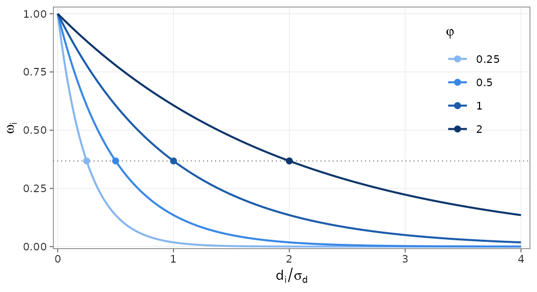
Four decreasing exponential curves of the weight against the distance divided by its standard deviation. Smaller localization values decrease faster.

Figure 1. Similarity weight as a function of the distance, for four localization values. Each curve crosses \(e^{-1}\) (dotted line) at \(d_i / \sigma_d = \varphi\) (points).

The two indexes therefore differ only in \(d_i\). Both, and the Mahalanobis distance that we use below for comparison, are quadratic forms of the difference \(\Delta_i = x_i - x_q\) between the standardized predictors:

\[ d_i^2 = \Delta_i^\top M \, \Delta_i, \]

Distance	\(M\)	Shape of the neighborhood	In lwpls
Euclidean	\(I\)	sphere	`similarity = "euclidean"`
Mahalanobis	\(S^{-1}\)	ellipsoid along the correlations of \(X\)	no
Covariance-based	\(\Gamma \Gamma^\top\)	slab perpendicular to \(\Gamma\)	`similarity = "covariance"`

Euclidean distance

Write the covariance matrix of the standardized predictors as \(S = \sum_k \lambda_k v_k v_k^\top\), with principal components \(v_k\) and variances \(\lambda_k\). The Euclidean distance is

\[ d_i^2 = \lVert \Delta_i \rVert^2 = \sum_k \left(v_k^\top \Delta_i\right)^2 . \]

Every direction enters the sum with the same coefficient, but for two random samples the term of component \(k\) is \(2 \lambda_k\) on average. The distance is therefore dominated by the largest sources of variation in \(X\), whether they are related to the outcome or not. In spectra, these are often baseline shifts, scattering or interfering compounds. The Euclidean distance does not use the outcome at all.

The Mahalanobis distance, \(M = S^{-1}\), divides each term by \(\lambda_k\) so that every component counts equally. It is often what “covariance-based distance” means, but it uses the covariance among the predictors. It is not available in lwpls: with more wavelengths than samples \(S\) cannot be inverted, and it inflates the components of smallest variance, which are mostly noise.

Covariance-based distance

Covariance-based LW-PLS (CbLW-PLS; Hazama and Kano, 2015) uses the covariance between the predictors and the outcome. With centered \(X\) and \(y\), the unit vector \(w\) that maximizes \(\operatorname{cov}(Xw, y) \propto w^\top X^\top y\) is, by the Cauchy–Schwarz inequality \(w^\top X^\top y \le \lVert w \rVert \, \lVert X^\top y \rVert\),

\[ \Gamma = \frac{X^\top y}{\lVert X^\top y \rVert}. \]

\(\Gamma\) is the first weight vector of a PLS model and \(t = X\Gamma\) is its first score. The distance is measured along this direction only:

\[ d_i = \left| \Gamma^\top (x_i - x_q) \right| = |t_i - t_q| . \]

A one-component PLS model predicts \(\hat y = \bar y + b \, t\), so \(|\hat y_i - \hat y_q| = |b| \, d_i\). The factor \(|b|\) cancels in \(d_i / \sigma_d\): the covariance-based weights are those obtained from the distance between the predictions of a one-component global PLS model. The neighbors of the query are the training samples that this simple model predicts to have a similar outcome.

Since \(M = \Gamma\Gamma^\top\) has rank one, all the directions perpendicular to \(\Gamma\) are ignored: samples far from the query in \(X\) are full neighbors if they have the same score \(t\). With several outcomes (or classes, coded as indicators), \(\Gamma = X^\top Y / \lVert X^\top Y \rVert_F\) has one column per outcome and \(d_i = \lVert \Gamma^\top (x_i - x_q) \rVert\). Robust models (robust = TRUE) compute \(\Gamma\) with the initial weights of partial robust M-regression, so that outliers do not distort it.

The three neighborhoods side by side

Two correlated predictors and a nonlinear outcome are enough to see the shapes:

set.seed(2026)
n <- 250
x1 <- rnorm(n)
x2 <- 0.75 * x1 + sqrt(1 - 0.75^2) * rnorm(n)
y <- sin(1.5 * x1) + 0.3 * x2 + rnorm(n, sd = 0.1)
x <- scale(cbind(x1, x2))

gamma <- crossprod(x, y - mean(y))
gamma <- drop(gamma / sqrt(sum(gamma^2)))
gamma
#>        x1        x2 
#> 0.7601460 0.6497523

query <- c(0.6, 0.2)
distance <- list(
  "Euclidean" = function(z) sqrt(rowSums(sweep(z, 2, query)^2)),
  "Mahalanobis" = function(z) sqrt(mahalanobis(z, query, cov(x))),
  "Covariance-based" = function(z) abs(drop(sweep(z, 2, query) %*% gamma))
)

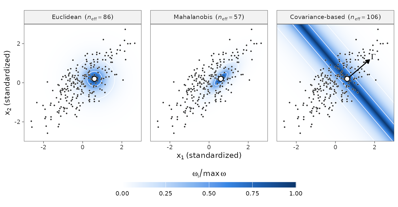
Three maps of the weights over the two predictors. Euclidean weights form circles around the query, Mahalanobis weights form ellipses along the correlation of the predictors, and covariance-based weights form a band perpendicular to the arrow Gamma.

Figure 2. Weights of the three distances around the same query (white point) with \(\varphi = 0.5\), relative to the largest one, with contour lines at 0.1 and 0.5. The arrow is \(\Gamma\), and \(n_\text{eff} = (\sum \omega_i)^2 / \sum \omega_i^2\) is the effective number of neighbors.

The Euclidean neighborhood is a circle. The Mahalanobis neighborhood stretches along the main axis of the cloud, the direction of largest variance of \(X\). The covariance-based neighborhood is a band across that same axis: here \(\Gamma\) points along it, because that is where the predictors covary with \(y\), and differences along \(\Gamma\) are exactly what the covariance-based distance measures.

When the covariance-based index helps

The simulated spectra below contain three sources of variation: an analyte band whose absorbance saturates with the concentration (the outcome), so that the relationship is nonlinear; a large interfering band; and baseline offsets and slopes. Only the analyte is related to the outcome, while most of the variance of \(X\) comes from the interferent and the baseline.

wavelength <- seq(1100, 1700, by = 5)
band <- function(center, width) exp(-0.5 * ((wavelength - center) / width)^2)

simulate_spectra <- function(n) {
  concentration <- runif(n, 0.05, 1)
  absorbance <- 1 - exp(-2.5 * concentration)
  interferent <- runif(n, 0, 1.5)
  offset <- rnorm(n, sd = 0.15)
  slope <- rnorm(n, sd = 0.1)
  x <- outer(0.8 * absorbance, band(1460, 22)) +
    outer(interferent, band(1330, 70)) +
    outer(offset, rep(1, length(wavelength))) +
    outer(slope, (wavelength - 1400) / 300) +
    matrix(rnorm(n * length(wavelength), sd = 0.004), n)
  colnames(x) <- paste0("nm", wavelength)
  list(x = x, y = concentration)
}

set.seed(7)
train <- simulate_spectra(300)
test <- simulate_spectra(300)

We compute \(\Gamma\) on the standardized training spectra, as lwpls does, and measure how well the score \(t = X\Gamma\) tracks the outcome:

x_train <- scale(train$x)
gamma_spectra <- crossprod(x_train, train$y - mean(train$y))
gamma_spectra <- drop(gamma_spectra / sqrt(sum(gamma_spectra^2)))
cor(drop(x_train %*% gamma_spectra), train$y)
#> [1] 0.8557298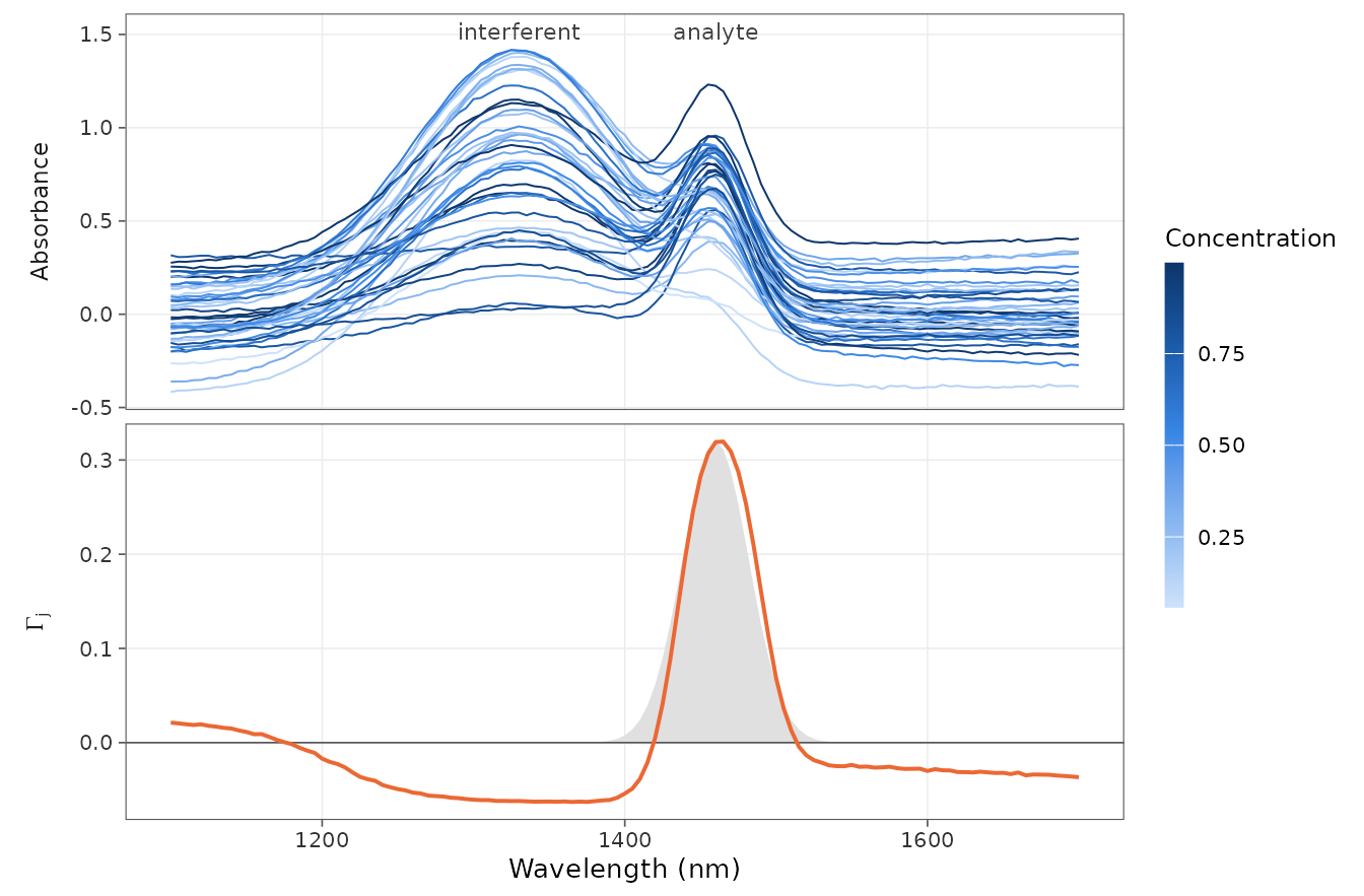

Top panel: simulated spectra with a broad interfering band near 1330 nm and a narrower analyte band near 1460 nm. Bottom panel: Gamma, which peaks at the analyte band and is close to zero elsewhere.

Figure 3. Top: 40 training spectra, colored by their concentration. Bottom: the covariance direction \(\Gamma\), with the analyte band in gray. \(\Gamma\) peaks on the analyte band; its small, flat loading elsewhere comes from a chance correlation of the outcome with the interferent and the baseline.

We then fit LW-PLS with both indexes over a range of localization values and compute the test RMSE. A very large localization gives nearly equal weights, that is, a global PLS model, which we use as a reference:

rmse_by_localization <- function(train, test, num_comp, localization) {
  grid <- expand.grid(localization = localization,
                      similarity = c("euclidean", "covariance"),
                      stringsAsFactors = FALSE)
  grid$rmse <- mapply(function(phi, index) {
    fit <- lwpls_fit(train$x, train$y, num_comp = num_comp,
                     localization = phi, similarity = index)
    sqrt(mean((test$y - predict(fit, test$x)$.pred)^2))
  }, grid$localization, grid$similarity)
  grid
}

global_rmse <- function(train, test, num_comp) {
  fit <- lwpls_fit(train$x, train$y, num_comp = num_comp, localization = 1e6)
  sqrt(mean((test$y - predict(fit, test$x)$.pred)^2))
}

localization_grid <- 10^seq(-1.5, 1, length.out = 14)
spectra_rmse <- rmse_by_localization(train, test, num_comp = 4, localization_grid)
spectra_global <- global_rmse(train, test, num_comp = 4)

# Best localization of each index
do.call(rbind, lapply(split(spectra_rmse, spectra_rmse$similarity),
                      function(d) d[which.min(d$rmse), ]))
#>            localization similarity       rmse
#> covariance    0.1858792 covariance 0.02859642
#> euclidean     0.1858792  euclidean 0.05997618
spectra_global
#> [1] 0.0804894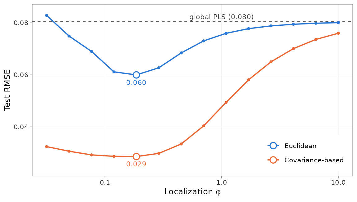

Test RMSE against localization on a log scale. The covariance-based curve stays below the Euclidean curve everywhere, with a minimum about half as large. Both approach the global PLS error for large localization.

Figure 4. Test RMSE of LW-PLS with 4 components on the simulated spectra. Open circles mark the best localization of each index, with its RMSE; the dashed line is the global PLS model.

The covariance-based index halves the error of the Euclidean index. The weights of a single query show why. lwpls_local() reports the effective number of neighbors of each prediction, and the weights themselves follow from the formulas above:

query_id <- which.min(abs(test$y - 0.5))
query_x <- test$x[query_id, , drop = FALSE]
z_query <- (drop(query_x) - attr(x_train, "scaled:center")) /
  attr(x_train, "scaled:scale")

d_euclidean <- sqrt(rowSums(sweep(x_train, 2, z_query)^2))
d_covariance <- abs(drop(sweep(x_train, 2, z_query) %*% gamma_spectra))
relative_weights <- function(d, phi) exp(-(d - min(d)) / (sd(d) * phi))

query_fits <- lapply(c(euclidean = "euclidean", covariance = "covariance"),
                     function(index) {
  lwpls_fit(train$x, train$y, num_comp = 4, localization = 0.2,
            similarity = index)
})
sapply(query_fits, function(fit) lwpls_local(fit, query_x)$reliability$n_eff)
#>  euclidean covariance 
#>   13.02410   71.92348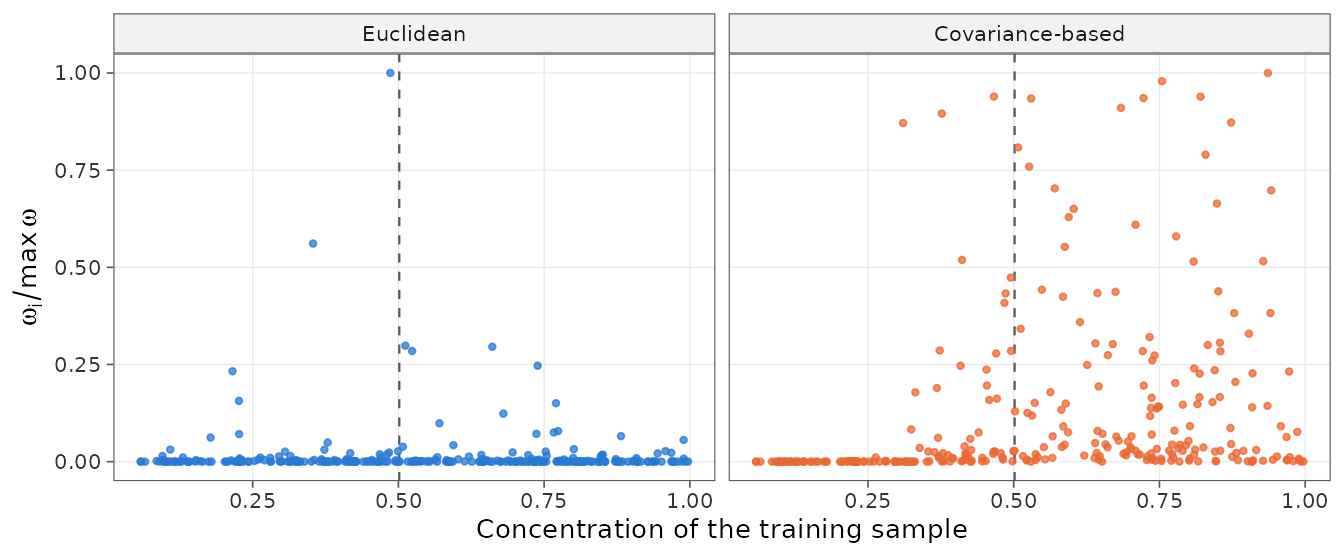

Two scatter plots of the weights against the concentration of the training samples. Euclidean weights are high for a few samples spread over all concentrations. Covariance-based weights are zero below a concentration of 0.3 and spread over the samples above.

Figure 5. Weights of the training samples for one test spectrum with a concentration of 0.5 (dashed line), against their own concentration (\(\varphi = 0.2\), weights relative to the largest one).

The Euclidean neighbors are close to the query in interferent and baseline, not in concentration, so they are spread over the whole concentration range. The covariance-based index gives almost no weight to the samples below 0.3. Its neighborhood is still broad and asymmetric, for two reasons: saturation compresses the differences between high concentrations along \(\Gamma\), and \(\Gamma\) keeps a small loading on the interferent and the baseline (Figure 3).

When the covariance-based index fails

\(\Gamma\) only captures the linear covariance between the predictors and the outcome. When the outcome is a symmetric function of a predictor, that covariance vanishes: with \(x_1\) standard normal and \(y = x_1^2\), \(\operatorname{cov}(x_1, y) = E[x_1^3] = 0\). \(\Gamma\) is then set by chance correlations in the training set.

simulate_symmetric <- function(n) {
  x <- matrix(rnorm(n * 5), n, dimnames = list(NULL, paste0("x", 1:5)))
  list(x = x, y = x[, 1]^2 + rnorm(n, sd = 0.2))
}

set.seed(11)
train_sym <- simulate_symmetric(300)
test_sym <- simulate_symmetric(300)

x_sym <- scale(train_sym$x)
gamma_sym <- crossprod(x_sym, train_sym$y - mean(train_sym$y))
gamma_sym <- drop(gamma_sym / sqrt(sum(gamma_sym^2)))
round(gamma_sym, 2)
#>    x1    x2    x3    x4    x5 
#>  0.46  0.10 -0.06  0.74 -0.48
cor(drop(x_sym %*% gamma_sym), train_sym$y)
#> [1] 0.148371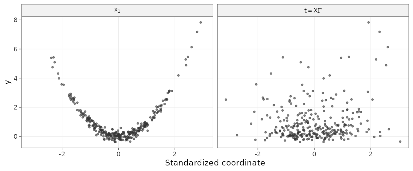

Left: a clear parabola of the outcome against x1. Right: the outcome against the score t shows no clear pattern.

Figure 6. The outcome against \(x_1\), the predictor it depends on (left), and against the score \(t = X\Gamma\) that the covariance-based distance uses (right).

symmetric_rmse <- rmse_by_localization(train_sym, test_sym, num_comp = 2,
                                       localization_grid)
symmetric_global <- global_rmse(train_sym, test_sym, num_comp = 2)
do.call(rbind, lapply(split(symmetric_rmse, symmetric_rmse$similarity),
                      function(d) d[which.min(d$rmse), ]))
#>            localization similarity      rmse
#> covariance    0.4506570 covariance 1.1174741
#> euclidean     0.2894266  euclidean 0.4598991
symmetric_global
#> [1] 1.322462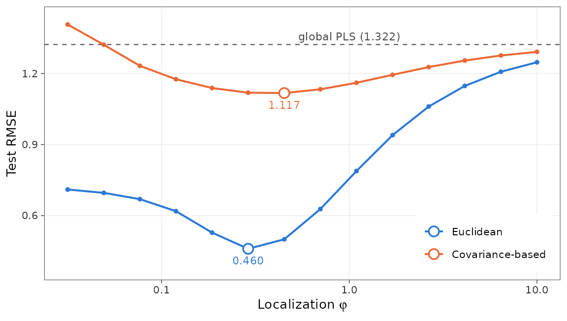

Test RMSE against localization on a log scale. The Euclidean curve reaches a much lower minimum than the covariance-based curve, which stays close to the global PLS error.

Figure 7. Test RMSE of LW-PLS with 2 components for \(y = x_1^2\). Open circles mark the best localization of each index, with its RMSE; the dashed line is the global PLS model.

The Euclidean neighborhoods still follow \(x_1\), while the covariance-based ones mostly follow noise: the covariance-based error is more than twice the Euclidean one, and only a little below that of the global model. The same happens whenever the local behavior depends on a direction that the global covariance \(X^\top y\) does not capture, for example regimes defined by other constituents of the samples (such as matrix effects in emission spectroscopy).

Choosing in practice

Look at \(\Gamma\) first. Computing it takes one line (see above). If it resembles the spectral signature of the property to predict and the score \(t = X\Gamma\) is well correlated with the outcome, the covariance-based index is likely to help. If \(\Gamma\) looks like noise, or the correlation is weak, prefer the Euclidean index.
The covariance-based index suits data in which most of the variance of \(X\) is unrelated to the outcome (interferents, baseline, scattering, temperature) and the outcome changes monotonically with the relevant signal, as in many NIR, Raman or LIBS calibrations.
The Euclidean index suits nonmonotonic relationships, local behavior driven by directions other than \(X^\top y\), and data whose irrelevant variation has already been removed by preprocessing (SNV, derivatives), since the Euclidean distance then reflects the relevant variation. It also does not depend on the outcome, so it cannot be misled by chance correlations.
Tune both. The best localization differs between the indexes (Figures 4 and 7), so similarity should be tuned together with localization and num_comp, as shown in vignette("lwpls").

References

Kim, S., Kano, M., Nakagawa, H. and Hasebe, S. (2011). Estimation of active pharmaceutical ingredients content using locally weighted partial least squares and statistical wavelength selection. International Journal of Pharmaceutics, 421(2), 269–274.
Hazama, K. and Kano, M. (2015). Covariance-based locally weighted partial least squares for high-performance adaptive modeling. Chemometrics and Intelligent Laboratory Systems, 146, 55–62.