Robust SIMCA Classification (RSIMCA)

Robust soft independent modeling of class analogy (RSIMCA) of Vanden Branden and Hubert (2005): a robust PCA model (robpca()) of each class, and the assignment of each observation to the class whose model is the closest, from its score and orthogonal distances. It applies to high-dimensional data such as whole spectra, and outlying spectra of the training data have little influence on the class models.

Usage

rsimca(
  x,
  group,
  ncomp = NULL,
  kmax = 10,
  alpha = 0.75,
  gamma = 0.5,
  squared = TRUE,
  var_explained = 0.8,
  prior = NULL,
  ndir = 250,
  nsamp = 500
)

Arguments

x: A numeric matrix or data frame of the predictors (spectra), one observation per row.
group: The classes of the observations: a factor, or a vector converted to one. Each class needs at least 5 observations.
ncomp: The number of components of the robust PCA of each class: a single number for all the classes, one per class (in the order of the levels of group, or named by them), or NULL (default) to let robpca() choose them from var_explained.
kmax: The largest number of components of the robust PCA. Default is 10.
alpha: The robustness parameter of robpca(): the fraction of observations of each class assumed to be regular, between 0.5 and 1. Default is 0.75.
gamma: The weight of the orthogonal distances in the classification rule, between 0 and 1. Default is 0.5.
squared: If TRUE (default), the rule combines the squared scaled distances (R2 of the paper); otherwise the scaled distances (R1).
var_explained: The proportion of variance explained used by robpca() to choose the number of components when ncomp is NULL. Default is 0.8.
prior: The membership (prior) probabilities of the classes, used to weight the overall misclassification rate, in the order of the levels of group (or named by them). Default is the proportions of the regular training observations in each class.
ndir, nsamp: The number of random directions of the outlyingness and of random subsets of FAST-MCD in robpca(). Defaults are 250 and 500.

Value

An object of class specproc_rsimca, a list with:

models: the robpca() model of each class.
ncomp: the number of components of each class model.
distances: a tibble with the combined distance $D_j$ of each training observation to each class.
group: the classes of the training observations, and fitted, the classes assigned to them.
weights: 1 for the observations regular in the model of their class, 0 for the others.
outlying: TRUE for the observations outlying for every class.
misclassification: a tibble with the misclassification rate of each class on its regular training observations, and the overall rate.
prior, gamma, squared, levels, alpha.

Use predict() for the classes and distances of new observations.

Details

Each class is modeled by robpca() with ncomp components (or the number chosen by robpca() from var_explained). For an observation $x$ and the model of class $j$, the score distance $SD_j(x)$ and the orthogonal distance $OD_j(x)$ are divided by their cut-offs, so that 1 marks the boundary of the class. The observation is assigned to the class with the smallest combined distance $$D_j(x) = \gamma \left(\frac{OD_j(x)}{c_{OD,j}}\right)^2 + (1 - \gamma) \left(\frac{SD_j(x)}{c_{SD,j}}\right)^2$$ (rule R2 of the paper), or with the distances instead of their squares when squared = FALSE (rule R1). gamma weights the orthogonal distances against the score distances.

An observation whose two scaled distances exceed 1 for every class is an outlier for all of them (outlying): it is still assigned to the closest class, but probably belongs to none.

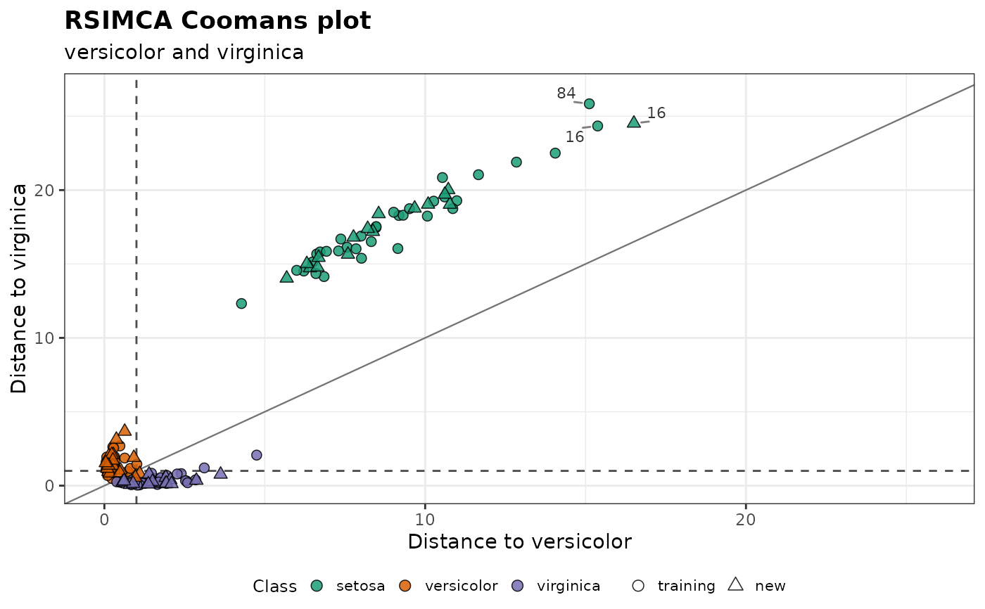
plot_coomans() draws the distances to two classes against each other (Coomans plot), and plot_outlier_map(fit$models[[j]]) the score and orthogonal distances to the robust PCA model of class j.

The misclassification rates are estimated on the regular observations of the training data (those regular in the robust PCA of their class), and the overall rate is weighted by the membership probabilities, by default the proportions of these observations in each class. They tend to underestimate the error: estimate it on test data or by cross-validation.

In tidymodels, rsimca() is the "rsimca" engine of the simca() parsnip model, where ncomp (num_comp), gamma and squared can be tuned.

Differences from the paper. The number of components of each class is given (ncomp) or chosen by robpca() from the proportion of variance explained, instead of by robust cross-validation (PRESS).

This is an independent implementation of the published description. robpca() uses random directions and subsets, so use set.seed() for reproducible results.

References

Vanden Branden, K., Hubert, M. (2005). Robust classification in high dimensions based on the SIMCA method. Chemometrics and Intelligent Laboratory Systems, 79(1-2):10-21.
Hubert, M., Rousseeuw, P.J., Vanden Branden, K. (2005). ROBPCA: a new approach to robust principal component analysis. Technometrics, 47(1):64-79.

Author

Christian L. Goueguel

Examples

# iris: train on 100 flowers, predict the 50 others
set.seed(1)
train <- sample(nrow(iris), 100)
fit <- rsimca(iris[train, 1:4], iris$Species[train], ncomp = 2)
fit
#> Robust SIMCA (RSIMCA)
#> 
#> Observations:   100 (15 outliers in their class, 14 in all classes)
#> Variables:      4
#> Classes:        setosa (2 comp.), versicolor (2 comp.), virginica (2 comp.)
#> Rule:           gamma = 0.5, squared scaled distances
#> 
#> Misclassification of the regular training observations:
#> # A tibble: 4 × 3
#>   class          n  error
#>   <chr>      <int>  <dbl>
#> 1 setosa        27 0     
#> 2 versicolor    28 0.0357
#> 3 virginica     30 0     
#> 4 overall       85 0.0118
table(predicted = predict(fit, iris[-train, 1:4]), true = iris$Species[-train])
#>             true
#> predicted    setosa versicolor virginica
#>   setosa         16          0         0
#>   versicolor      0         17         0
#>   virginica       0          2        15
plot_coomans(fit, classes = c("versicolor", "virginica"),
             newdata = iris[-train, 1:4], group = iris$Species[-train])