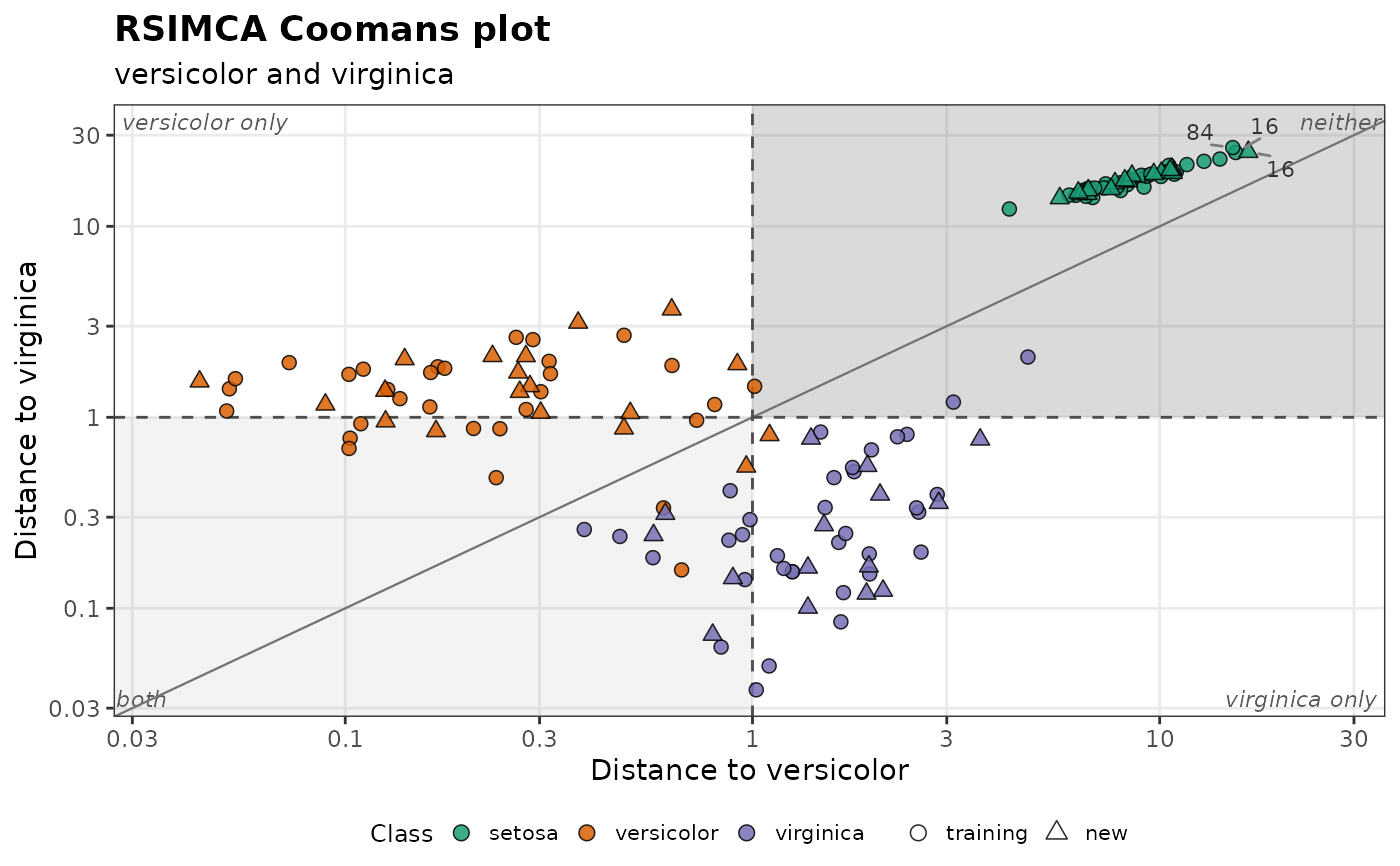
Coomans Plot of a Robust SIMCA Model

Plots the distance of each observation to one class of a model fitted by rsimca() against its distance to another class (Coomans plot), with the class boundaries and the classification boundary. It shows which observations belong to one class, to both, or to neither, and which are misclassified.

Usage

plot_coomans(
  object,
  newdata = NULL,
  group = NULL,
  classes = NULL,
  labels = 3,
  log = FALSE,
  shade = FALSE,
  title = NULL,
  ...
)

Arguments

object: An object returned by rsimca().
newdata: Optional new observations to add to the plot (a numeric matrix or data frame with the training variables).
group: Optional classes of newdata, to fill their points.
classes: The two classes to plot, on the horizontal and vertical axes. Default is the first two classes of the model.
labels: The number of observations farthest from both classes to label, among those beyond 1 for both (by their row names, or row numbers). Default is 3; use 0 for no labels.
log: If TRUE, use logarithmic axes, which spread out the observations close to the classes when others are far away. Default is FALSE.
shade: If TRUE, shade the regions of the observations close to both classes and to neither, and name the four regions. Default is FALSE.
title: The plot title.
...: Further arguments passed to ggplot2::geom_point() to style the points, such as alpha (default 0.85), size (2.2), stroke (0.4) or colour (the outline, "black"). size can also be a numeric vector with one value per observation (the training observations, then those of newdata), to vary the size of the points, with a legend.

Value

A ggplot object.

Details

The distances are the combined distances \(D_j\) of the classification rule of rsimca(), built from the score and orthogonal distances to the robust PCA model of each class, divided by their cut-offs. The dashed lines are at 1: an observation beyond 1 for a class is beyond at least one of the cut-offs of this class, and an observation within both cut-offs of a class is within 1. The diagonal is the classification boundary: the observations above it are assigned to the class of the horizontal axis, those below it to the class of the vertical axis.

The four corners of the plot hold the observations close to the class of the horizontal axis only (top left), to the class of the vertical axis only (bottom right), to both (bottom left, where the classes overlap), and to neither (top right, outliers for both classes, or, with more than two classes, members of another class).

The points are filled by their class: the training class for the training observations, and for new observations (newdata, triangles) the classes given in group, or "unknown". Observations of a class on the wrong side of the diagonal are misclassified.

References

Vanden Branden, K., Hubert, M. (2005). Robust classification in high dimensions based on the SIMCA method. Chemometrics and Intelligent Laboratory Systems, 79(1-2):10-21.

Author

Christian L. Goueguel

Examples

# iris: train on 100 flowers, predict the 50 others
set.seed(1)
train <- sample(nrow(iris), 100)
fit <- rsimca(iris[train, 1:4], iris$Species[train], ncomp = 2)
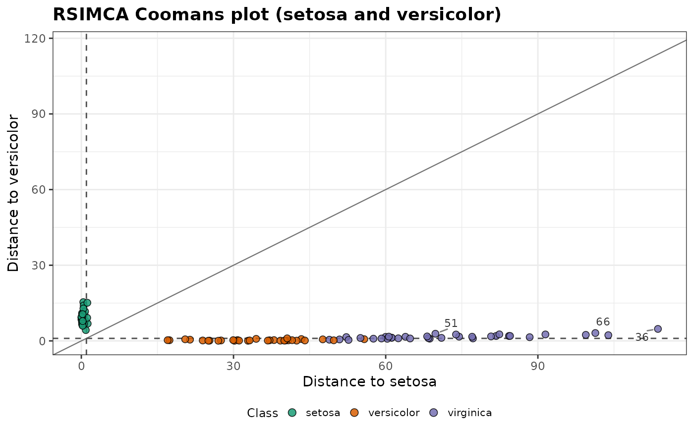
# the first two classes, setosa and versicolor
plot_coomans(fit)

# versicolor and virginica, with the 50 new flowers (triangles)
plot_coomans(fit, classes = c("versicolor", "virginica"),
             newdata = iris[-train, 1:4], group = iris$Species[-train],
             log = TRUE, shade = TRUE)