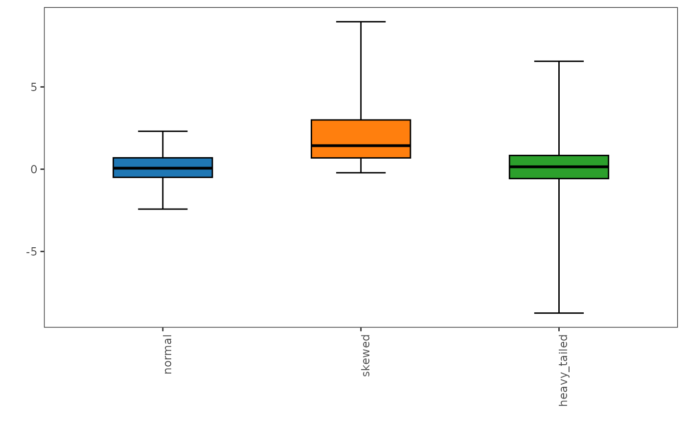
This function implements the generalized boxplot, a robust data visualization technique designed to effectively represent skewed and heavy-tailed distributions, as proposed by Bruffaerts et al. (2014).
Usage
generalized_boxplot(
  x,
  alpha = 2 * stats::pnorm(-4 * stats::qnorm(0.75)),
  p = 0.9,
  plot = TRUE,
  id = NULL,
  group = NULL,
  scales = c("free_y", "fixed"),
  points = c("outliers", "all", "none"),
  label_outliers = FALSE,
  show_n = TRUE,
  show_mean = FALSE,
  annotate = NULL,
  horizontal = FALSE,
  log = FALSE,
  fill = "grey85",
  xlab = NULL,
  ylab = NULL,
  title = NULL,
  caption = TRUE,
  base_size = 11,
  x_labels_angle = 0,
  box_width = 0.5,
  notch = FALSE,
  notch_width = 0.5,
  staple_width = 0.5,
  xlabels.angle = deprecated(),
  xlabels.vjust = deprecated(),
  xlabels.hjust = deprecated(),
  box.width = deprecated(),
  notchwidth = deprecated(),
  staplewidth = deprecated()
)
Arguments
- x
A data frame (or matrix) of numeric variables, with optionally the columns
idandgroup.- alpha
The expected proportion of observations outside the fences in clean data, between 0 and 1. Default is \(2\,\Phi(-4 z_{0.75}) \approx 0.007\), as Tukey's boxplot for normal data.
- p
The quantile order, between 0.5 and 1, of the estimation of g and h. Default is 0.9 (a breakdown point of 10%).
- plot
A logical value indicating whether to plot the boxplot (default is
TRUE) or to return its statistics.- id
Optional column of
x(unquoted or as a string) identifying the observations, such as sample names: it names the outlying observations in theoutlierstable and withlabel_outliers.- group
Optional column of
x(unquoted or as a string) of groups, such as sites or treatments: the boxes of each group are drawn side by side, with their own statistics. Rows with a missing group are left out.- scales
"free_y"(default), one panel per variable with its own value axis, or"fixed", a common value axis.- points
The observations drawn:
"outliers"(default), the outlying ones;"all"; or"none".- label_outliers
A logical: label the outlying observations with their
id, else their row number (FALSE, default). The labels are moved apart so that they do not overlap; where many outliers crowd together, some are left unlabeled.- show_n
A logical: write the number of values below each box (
TRUE, default).- show_mean
A logical: mark the mean of each box with a diamond (
FALSE, default).- annotate
Statistics added to each box (none by default): some of
"shape","outliers","fences","median","spread","location","test"and"missing", or"all"(see Details).- horizontal
A logical: horizontal boxes (
FALSE, default), suited to many variables or long names.- log
A logical: a logarithmic value axis (
FALSE, default), for variables spanning orders of magnitude. The statistics are those of the data, not of their logarithm.- fill
The fill color of the boxes (default
"grey85"), or one color per group (or per variable withoutgroup).- xlab, ylab
The titles of the axis of the variables (or groups) and of the value axis. Default is none.
- title
The plot title. A long title is split into a title and a subtitle.
- caption
TRUE(default), a caption naming the boxplot and its whiskers;FALSE, no caption; or a caption of your own.- base_size
The size of the text, in points. Default is 11.
- x_labels_angle
The angle (in degrees) of the labels below the boxes. Default is 0 (horizontal).
- box_width
The width of the boxes (default 0.5).
- notch
A logical value indicating whether to draw notches (default is
FALSE): the notch spans the median \(\pm 1.58\,\text{IQR}/\sqrt{n}\) (McGill et al., 1978); two medians whose notches do not overlap differ roughly at the 5% level.- notch_width
The width of the notch relative to the box (default 0.5).
- staple_width
The width of the staples at the ends of the whiskers, relative to the box (default 0.5).
- xlabels.angle, xlabels.vjust, xlabels.hjust, box.width, notchwidth, staplewidth
![[Deprecated]](figures/lifecycle-deprecated.svg) Use
Use x_labels_angle,box_width,notch_widthandstaple_width; the justification of the labels now follows their angle.
Value
If
plot = TRUE, aggplot2object.If
plot = FALSE, a list of tibbles:stats,outliersand, withgroup,tests, as inadjusted_boxplot(), with the estimatedgandhinstead of the medcouple, andalpha * nexpected outlying values.
Details
This method extends the adjusted boxplot method by leveraging the flexible Tukey's g-and-h parametric distribution to model the underlying data structure, particularly for asymmetric or long-tailed datasets, providing a more nuanced and informative summary of the data's central tendency, spread, and potential outliers.
The data \(x_i\) are first mapped, preserving their ranks, into (0, 1)
by \(r_i = (\tilde{x}_i - \min_j \tilde{x}_j + 0.1) /
(\max_j \tilde{x}_j - \min_j \tilde{x}_j + 0.2)\), with
\(\tilde{x}_i = (x_i - \text{median}) / \text{IQR}\), and then onto the
real line by \(w_i = \Phi^{-1}(r_i)\). The \(w_i\), standardized by
their median and their interquartile range divided by
\(z_{0.75} - z_{0.25} = 1.349\), are fitted by a Tukey g-and-h
distribution, whose skewness \(g\) and tail heaviness \(h\) are
estimated from the quantiles of orders \(p\) and \(1 - p\). The fences
are the quantiles of orders \(\alpha/2\) and \(1 - \alpha/2\) of the
fitted distribution, mapped back to the scale of the data: a proportion
\(\alpha\) of the observations of a clean distribution, of whatever
skewness and tails, is expected outside. The default \(\alpha =
2\,\Phi(-4 z_{0.75}) \approx 0.7\%\), the rate of Tukey's boxplot for normal
data, is that of the authors' implementation (the Stata command robbox
of Jann, Verardi and Vermandele). The fences are not inside the box, and
the whiskers end at the most extreme observations within the fences.
The outlying observations are therefore atypical at the rate \(\alpha\): about \(\alpha n\) of them are expected in clean data, so that with a large \(\alpha\) (such as 5%) many flagged observations are not errors. As \(h\) may be negative (tails lighter than normal), where the g-and-h transform turns back before the \(\alpha/2\) quantile the fence is its extreme value.
The layout, the points, the annotations and the options for publication
figures are those of adjusted_boxplot(): see its details.
References
Bruffaerts, C., Verardi, V., Vermandele, C. (2014). A generalized boxplot for skewed and heavy-tailed distributions. Statistics and Probability Letters 95(C):110–117
Verardi, V., Vermandele, C. (2016). Outlier identification for skewed and/or heavy-tailed unimodal multivariate distributions. Journal de la Société Française de Statistique, 157(2):90–114
Examples
data(forageLIBS)
minerals <- forageLIBS[c("Measurement", "Ca", "Mg", "P", "K", "S")]
# mineral contents, each on its own axis, the outlying samples named: a
# figure of a journal page width
p <- generalized_boxplot(minerals, id = Measurement, label_outliers = TRUE,
ylab = "Content (%)", base_size = 8)
p
 # ggplot2::ggsave("minerals.pdf", p, width = 175, height = 70, units = "mm")
# the statistics and the outlying samples
res <- generalized_boxplot(minerals, id = Measurement, plot = FALSE)
res$stats
#> # A tibble: 5 × 22
#> variable n n_missing lower q1 median q3 upper lower_fence
#> <fct> <int> <int> <dbl> <dbl> <dbl> <dbl> <dbl> <dbl>
#> 1 Ca 368 0 0.337 0.515 0.629 0.772 1.12 0.334
#> 2 Mg 368 0 0.0919 0.172 0.204 0.240 0.342 0.0850
#> 3 P 368 0 0.135 0.219 0.260 0.300 0.436 0.132
#> 4 K 368 0 0.829 1.72 2.01 2.38 3.56 0.668
#> 5 S 366 2 0.13 0.17 0.2 0.23 0.31 0.122
#> # ℹ 13 more variables: upper_fence <dbl>, notch_lower <dbl>, notch_upper <dbl>,
#> # g <dbl>, h <dbl>, median_lower <dbl>, median_upper <dbl>, iqr <dbl>,
#> # rcv <dbl>, biweight <dbl>, mean <dbl>, n_outliers <int>,
#> # expected_outliers <dbl>
res$outliers
#> # A tibble: 27 × 5
#> variable row id value out
#> <fct> <int> <int> <dbl> <chr>
#> 1 Ca 182 121370 1.45 upper
#> 2 Ca 248 121094 0.173 lower
#> 3 Ca 252 121085 0.313 lower
#> 4 Ca 274 121096 0.292 lower
#> 5 Ca 306 121404 0.323 lower
#> 6 Ca 354 121580 1.2 upper
#> 7 Mg 98 121144 0.365 upper
#> 8 Mg 140 121151 0.359 upper
#> 9 Mg 167 121035 0.362 upper
#> 10 Mg 248 121094 0.0527 lower
#> # ℹ 17 more rows
# with a detection rate of 5%, about 18 of the 368 samples would be
# flagged per mineral even in clean data
generalized_boxplot(minerals, id = Measurement, alpha = 0.05, plot = FALSE)$stats
#> # A tibble: 5 × 22
#> variable n n_missing lower q1 median q3 upper lower_fence
#> <fct> <int> <int> <dbl> <dbl> <dbl> <dbl> <dbl> <dbl>
#> 1 Ca 368 0 0.38 0.515 0.629 0.772 1.03 0.375
#> 2 Mg 368 0 0.116 0.172 0.204 0.240 0.315 0.114
#> 3 P 368 0 0.16 0.219 0.260 0.300 0.393 0.160
#> 4 K 368 0 1.04 1.72 2.01 2.38 3.04 1.01
#> 5 S 366 2 0.14 0.17 0.2 0.23 0.28 0.133
#> # ℹ 13 more variables: upper_fence <dbl>, notch_lower <dbl>, notch_upper <dbl>,
#> # g <dbl>, h <dbl>, median_lower <dbl>, median_upper <dbl>, iqr <dbl>,
#> # rcv <dbl>, biweight <dbl>, mean <dbl>, n_outliers <int>,
#> # expected_outliers <dbl>
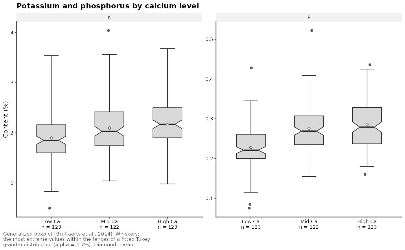
# potassium and phosphorus by calcium level, with notches and means: a
# figure of a journal column
minerals$Ca_level <- cut(minerals$Ca, quantile(minerals$Ca, 0:3 / 3),
labels = c("Low Ca", "Mid Ca", "High Ca"),
include.lowest = TRUE)
p <- generalized_boxplot(minerals[c("K", "P", "Ca_level")], group = Ca_level,
notch = TRUE, show_mean = TRUE, ylab = "Content (%)",
title = "Potassium and phosphorus by calcium level",
base_size = 8)
p
# ggplot2::ggsave("minerals.pdf", p, width = 175, height = 70, units = "mm")
# the statistics and the outlying samples
res <- generalized_boxplot(minerals, id = Measurement, plot = FALSE)
res$stats
#> # A tibble: 5 × 22
#> variable n n_missing lower q1 median q3 upper lower_fence
#> <fct> <int> <int> <dbl> <dbl> <dbl> <dbl> <dbl> <dbl>
#> 1 Ca 368 0 0.337 0.515 0.629 0.772 1.12 0.334
#> 2 Mg 368 0 0.0919 0.172 0.204 0.240 0.342 0.0850
#> 3 P 368 0 0.135 0.219 0.260 0.300 0.436 0.132
#> 4 K 368 0 0.829 1.72 2.01 2.38 3.56 0.668
#> 5 S 366 2 0.13 0.17 0.2 0.23 0.31 0.122
#> # ℹ 13 more variables: upper_fence <dbl>, notch_lower <dbl>, notch_upper <dbl>,
#> # g <dbl>, h <dbl>, median_lower <dbl>, median_upper <dbl>, iqr <dbl>,
#> # rcv <dbl>, biweight <dbl>, mean <dbl>, n_outliers <int>,
#> # expected_outliers <dbl>
res$outliers
#> # A tibble: 27 × 5
#> variable row id value out
#> <fct> <int> <int> <dbl> <chr>
#> 1 Ca 182 121370 1.45 upper
#> 2 Ca 248 121094 0.173 lower
#> 3 Ca 252 121085 0.313 lower
#> 4 Ca 274 121096 0.292 lower
#> 5 Ca 306 121404 0.323 lower
#> 6 Ca 354 121580 1.2 upper
#> 7 Mg 98 121144 0.365 upper
#> 8 Mg 140 121151 0.359 upper
#> 9 Mg 167 121035 0.362 upper
#> 10 Mg 248 121094 0.0527 lower
#> # ℹ 17 more rows
# with a detection rate of 5%, about 18 of the 368 samples would be
# flagged per mineral even in clean data
generalized_boxplot(minerals, id = Measurement, alpha = 0.05, plot = FALSE)$stats
#> # A tibble: 5 × 22
#> variable n n_missing lower q1 median q3 upper lower_fence
#> <fct> <int> <int> <dbl> <dbl> <dbl> <dbl> <dbl> <dbl>
#> 1 Ca 368 0 0.38 0.515 0.629 0.772 1.03 0.375
#> 2 Mg 368 0 0.116 0.172 0.204 0.240 0.315 0.114
#> 3 P 368 0 0.16 0.219 0.260 0.300 0.393 0.160
#> 4 K 368 0 1.04 1.72 2.01 2.38 3.04 1.01
#> 5 S 366 2 0.14 0.17 0.2 0.23 0.28 0.133
#> # ℹ 13 more variables: upper_fence <dbl>, notch_lower <dbl>, notch_upper <dbl>,
#> # g <dbl>, h <dbl>, median_lower <dbl>, median_upper <dbl>, iqr <dbl>,
#> # rcv <dbl>, biweight <dbl>, mean <dbl>, n_outliers <int>,
#> # expected_outliers <dbl>
# potassium and phosphorus by calcium level, with notches and means: a
# figure of a journal column
minerals$Ca_level <- cut(minerals$Ca, quantile(minerals$Ca, 0:3 / 3),
labels = c("Low Ca", "Mid Ca", "High Ca"),
include.lowest = TRUE)
p <- generalized_boxplot(minerals[c("K", "P", "Ca_level")], group = Ca_level,
notch = TRUE, show_mean = TRUE, ylab = "Content (%)",
title = "Potassium and phosphorus by calcium level",
base_size = 8)
p
 # ggplot2::ggsave("by_calcium.pdf", p, width = 85, height = 75, units = "mm")
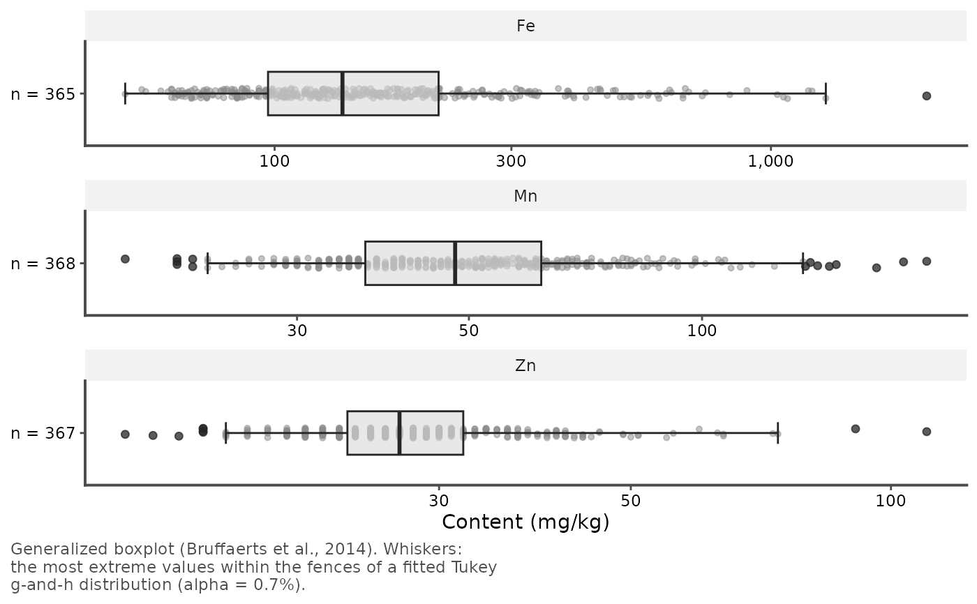
# trace elements on a logarithmic axis, horizontal, with all the samples
traces <- forageLIBS[c("Fe", "Mn", "Zn")]
generalized_boxplot(traces, log = TRUE, horizontal = TRUE, points = "all",
ylab = "Content (mg/kg)")
# ggplot2::ggsave("by_calcium.pdf", p, width = 85, height = 75, units = "mm")
# trace elements on a logarithmic axis, horizontal, with all the samples
traces <- forageLIBS[c("Fe", "Mn", "Zn")]
generalized_boxplot(traces, log = TRUE, horizontal = TRUE, points = "all",
ylab = "Content (mg/kg)")