Setup
import numpy as np
import pandas as pd
from matplotlib.patches import Arc
from scipy import stats

from pyEllipse import hotelling_coordinates, hotelling_parametersThis page states what pyEllipse computes, under which assumptions each result is exact, and how the functions map onto the formulas. The figures and the numbers quoted in the text are computed with pyEllipse when this page is built; expand “Show the code” to see how.
import numpy as np
import pandas as pd
from matplotlib.patches import Arc
from scipy import stats
from pyEllipse import hotelling_coordinates, hotelling_parametersimport matplotlib.pyplot as plt
from cycler import cycler
# Figure widths of most journals, in inches: single, 1.5 and double column
MM = 1 / 25.4
SINGLE, ONE_HALF, DOUBLE = 89 * MM, 140 * MM, 183 * MM
# Colour-blind-safe colours, used in this order; each figure also varies line style
# or marker shape, so it can be printed in grayscale
BLUE, ORANGE, AQUA, GREY = "#2a78d6", "#eb6834", "#1baf7a", "#808080"
plt.rcParams.update({
# Text and mathematics in the same sans-serif font, at the printed size
"font.family": "sans-serif",
"font.sans-serif": ["Arial", "Helvetica", "Liberation Sans", "DejaVu Sans"],
"font.size": 9,
"axes.labelsize": 9,
"xtick.labelsize": 8,
"ytick.labelsize": 8,
"legend.fontsize": 8,
"mathtext.fontset": "custom",
"mathtext.rm": "sans",
"mathtext.it": "sans:italic",
"mathtext.bf": "sans:bold",
"mathtext.sf": "sans",
"mathtext.cal": "sans:italic",
# Thin black axes, outward ticks, no grid
"axes.edgecolor": "black",
"axes.linewidth": 0.6,
"axes.spines.top": False,
"axes.spines.right": False,
"axes.prop_cycle": cycler(color=[BLUE, ORANGE, AQUA]),
"xtick.major.width": 0.6,
"ytick.major.width": 0.6,
"xtick.major.size": 3,
"ytick.major.size": 3,
"xtick.direction": "out",
"ytick.direction": "out",
"lines.linewidth": 1.2,
"legend.frameon": False,
# Saved figures keep the exact size set with figsize
"figure.constrained_layout.use": True,
# Vector output with embedded TrueType fonts; 600 dpi for raster formats
"pdf.fonttype": 42,
"ps.fonttype": 42,
"svg.fonttype": "none",
"savefig.dpi": 600,
})Let \(\mathbf{X}\) be an \(n \times p\) matrix of component scores (PCA, PLS, ICA, …), with one row per observation. For the \(k\) selected components, \(\mathbf{x}_i \in \mathbb{R}^k\) denotes the scores of observation \(i\), and
\[ \bar{\mathbf{x}} = \frac{1}{n}\sum_{i=1}^{n} \mathbf{x}_i, \qquad \mathbf{S} = \frac{1}{n-1}\sum_{i=1}^{n} (\mathbf{x}_i - \bar{\mathbf{x}})(\mathbf{x}_i - \bar{\mathbf{x}})^\top \tag{1}\]
are their sample mean vector and sample covariance matrix, with the \(n - 1\) denominator of numpy.cov. Confidence levels are written \(1 - \alpha\), and \(F_{1-\alpha}(d_1, d_2)\), \(B_{1-\alpha}(a, b)\) and \(\chi^2_{1-\alpha}(d)\) are the \(1 - \alpha\) quantiles of the F, Beta and chi-square distributions.
The T-squared statistic of observation \(i\) is its squared Mahalanobis distance from the mean (Hotelling 1931):
\[ T^2_i = (\mathbf{x}_i - \bar{\mathbf{x}})^\top \mathbf{S}^{-1} (\mathbf{x}_i - \bar{\mathbf{x}}). \tag{2}\]
This is the value returned in hotelling_parameters(...)['Tsquared']. With k=2 it is computed on components pcx and pcy, otherwise on the first k components (see Section 5).
\(T^2_i\) measures how far an observation lies from the centre of the data, in units of the data’s own spread and correlation. It does not change under any invertible linear transformation \(\mathbf{y} = \mathbf{A}\mathbf{x} + \mathbf{b}\) of the scores: the covariance of \(\mathbf{y}\) is \(\mathbf{A}\mathbf{S}\mathbf{A}^\top\), and \((\mathbf{A}\mathbf{d})^\top (\mathbf{A}\mathbf{S}\mathbf{A}^\top)^{-1} (\mathbf{A}\mathbf{d}) = \mathbf{d}^\top \mathbf{S}^{-1} \mathbf{d}\). Rescaling or mixing the selected components therefore leaves T-squared unchanged.
An observation is flagged when its T-squared value exceeds a cutoff \(c\), the \(1 - \alpha\) quantile of the distribution of T-squared. That distribution depends on how the observation relates to the \(n\) observations used to compute \(\bar{\mathbf{x}}\) and \(\mathbf{S}\). For independent observations from a multivariate normal distribution, the exact distributions are:
| Observation | Distribution of \(T^2\) | In pyEllipse |
|---|---|---|
| One of the \(n\) observations used to compute \(\bar{\mathbf{x}}\) and \(\mathbf{S}\) | \(\frac{(n-1)^2}{n}\,\mathrm{Beta}\left(\frac{k}{2}, \frac{n-k-1}{2}\right)\) | method='beta' |
| Independent of \(\mathbf{S}\), measured from the true mean \(\boldsymbol{\mu}\) | \(\frac{k(n-1)}{n-k}\,F(k, n-k)\) | method='f' (default) |
| A new observation, independent of the \(n\) observations, measured from \(\bar{\mathbf{x}}\) | \(\frac{k(n+1)(n-1)}{n(n-k)}\,F(k, n-k)\) | not provided |
method='f')\[ c_F = \frac{k(n-1)}{n-k}\, F_{1-\alpha}(k, n-k) \tag{4}\]
This is Hotelling’s T-squared distribution with \(n - 1\) degrees of freedom (Hotelling 1931; Mardia, Kent, and Bibby 1979): if \(\mathbf{z} \sim N_k(\mathbf{0}, \boldsymbol{\Sigma})\) is independent of \(\mathbf{S}\), with \((n-1)\mathbf{S} \sim W_k(\boldsymbol{\Sigma}, n-1)\), then \(\mathbf{z}^\top \mathbf{S}^{-1} \mathbf{z} \sim \frac{k(n-1)}{n-k} F(k, n-k)\). Taking \(\mathbf{z} = \mathbf{x} - \boldsymbol{\mu}\) for an observation independent of \(\mathbf{S}\) gives the second row of Table 1. The same distribution describes \(n(\bar{\mathbf{x}} - \boldsymbol{\mu})^\top \mathbf{S}^{-1} (\bar{\mathbf{x}} - \boldsymbol{\mu})\), Hotelling’s one-sample statistic for the mean.
Equation 4 is the limit traditionally used for score plots in chemometrics (Jackson 1991; Brereton 2016), and the default of pyEllipse and of the HotellingEllipse R package, for backward compatibility. It is exact for neither of the two practical cases:
method='beta')\[ c_B = \frac{(n-1)^2}{n}\, B_{1-\alpha}\left(\frac{k}{2}, \frac{n-k-1}{2}\right) \tag{5}\]
When \(\mathbf{x}_i\) is one of the observations used to compute \(\bar{\mathbf{x}}\) and \(\mathbf{S}\), it is not independent of them, and \(n\,T^2_i/(n-1)^2\) follows exactly a \(\mathrm{Beta}(k/2, (n-k-1)/2)\) distribution (Gnanadesikan and Kettenring 1972; Tracy, Young, and Mason 1992). As a Beta variable never exceeds 1, \(T^2_i \le (n-1)^2/n\) for every observation, whatever the data. Equation 5 is therefore the exact limit for flagging outliers among the samples a PCA or PLS model was built on.
For a new observation \(\mathbf{x}\), independent of the \(n\) observations, \(\mathbf{x} - \bar{\mathbf{x}} \sim N_k(\mathbf{0}, \frac{n+1}{n}\boldsymbol{\Sigma})\) is independent of \(\mathbf{S}\), which gives the third row of Table 1. pyEllipse computes T-squared and its limits from a single set of scores, so it does not provide this limit. To monitor new samples, compute their T-squared with the mean and covariance of the calibration scores, and compare it with \(\frac{k(n+1)(n-1)}{n(n-k)} F_{1-\alpha}(k, n-k)\).
As \(n \to \infty\), all three distributions converge to \(\chi^2(k)\). The distribution='normal' option of confidence_ellipse uses this large-sample limit (Section 6).
k, level = 2, 0.95
n = np.arange(6, 201)
f_lim = k * (n - 1) / (n - k) * stats.f.ppf(level, k, n - k)
beta_lim = (n - 1) ** 2 / n * stats.beta.ppf(level, k / 2, (n - k - 1) / 2)
new_lim = (n + 1) / n * f_lim
chi2_lim = stats.chi2.ppf(level, k)

fig, ax = plt.subplots(figsize=(ONE_HALF, 75 * MM))
ax.plot(n, new_lim, color=AQUA, ls="-.", label="New observation (exact)")
ax.plot(n, f_lim, color=BLUE, label="F limit, method='f'")
ax.plot(n, beta_lim, color=ORANGE, ls="--", label="Beta limit, method='beta' (exact in-sample)")
ax.axhline(chi2_lim, color=GREY, lw=0.8, label=r"$\chi^2_{0.95}(2)$, limit as $n \to \infty$")
ax.plot(n, (n - 1) ** 2 / n, color=GREY, lw=0.8, ls=":",
        label=r"Largest in-sample $T^2$, $(n-1)^2/n$")
ax.set_xscale("log")
ax.set_xticks([6, 10, 20, 50, 100, 200], labels=["6", "10", "20", "50", "100", "200"])
ax.minorticks_off()
ax.set_xlim(6, 200)
ax.set_ylim(0, 20)
ax.set_yticks(range(0, 21, 5))
ax.set_xlabel(r"Number of observations, $n$")
ax.set_ylabel(r"95% limit of $T^2$")
ax.legend(loc="upper right")
plt.show()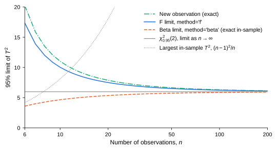
sizes = [6, 10, 20, 50, 100, 200]
idx = [list(n).index(s) for s in sizes]
pd.DataFrame({
    "n": sizes,
    "Beta limit": beta_lim[idx],
    "F limit": f_lim[idx],
    "New observation": new_lim[idx],
    "χ²(2)": chi2_lim,
    "Largest in-sample T²": [(s - 1) ** 2 / s for s in sizes],
}).round(2).style.hide(axis="index").format(precision=2)| n | Beta limit | F limit | New observation | χ²(2) | Largest in-sample T² |
|---|---|---|---|---|---|
| 6 | 3.60 | 17.36 | 20.25 | 5.99 | 4.17 |
| 10 | 4.66 | 10.03 | 11.04 | 5.99 | 8.10 |
| 20 | 5.36 | 7.50 | 7.88 | 5.99 | 18.05 |
| 50 | 5.75 | 6.51 | 6.64 | 5.99 | 48.02 |
| 100 | 5.87 | 6.24 | 6.30 | 5.99 | 98.01 |
| 200 | 5.93 | 6.11 | 6.14 | 5.99 | 198.00 |
The table below checks Table 1 by simulation: it draws data sets of \(n = 20\) observations of \(k = 2\) independent standard normal components, plus one new observation per data set, and reports the fraction of T-squared values above each 95% limit.
rng = np.random.default_rng(2026)
n_sim, k_sim, reps = 20, 2, 20_000
x = rng.standard_normal((reps, n_sim + 1, k_sim))
sample, new = x[:, :n_sim], x[:, n_sim]
d = sample - sample.mean(axis=1, keepdims=True)
s_inv = np.linalg.inv(np.einsum("rni,rnj->rij", d, d) / (n_sim - 1))
t2_in = np.einsum("rni,rij,rnj->rn", d, s_inv, d)
d_new = new - sample.mean(axis=1)
t2_new = np.einsum("ri,rij,rj->r", d_new, s_inv, d_new)

limits = {
    "Beta limit": (n_sim - 1) ** 2 / n_sim * stats.beta.ppf(0.95, k_sim / 2, (n_sim - k_sim - 1) / 2),
    "F limit": k_sim * (n_sim - 1) / (n_sim - k_sim) * stats.f.ppf(0.95, k_sim, n_sim - k_sim),
}
limits["New-observation limit"] = (n_sim + 1) / n_sim * limits["F limit"]
simulation = pd.DataFrame(
    {
        "In-sample observations": [np.mean(t2_in > c) for c in limits.values()],
        "New observations": [np.mean(t2_new > c) for c in limits.values()],
    },
    index=pd.Index(limits, name="95% limit"),
)
f_new_rate = simulation.loc["F limit", "New observations"]
simulation.style.format("{:.1%}")| In-sample observations | New observations | |
|---|---|---|
| 95% limit | ||
| Beta limit | 5.0% | 11.6% |
| F limit | 1.0% | 5.6% |
| New-observation limit | 0.8% | 5.0% |
In-sample observations exceed the Beta limit at the nominal 5% rate and the F limit far less often; new observations exceed the F limit 5.6% of the time and the new-observation limit at the nominal rate.
With \(k = 2\), the region where T-squared does not exceed the cutoff \(c\) is an ellipse:
\[ \mathcal{E} = \left\{\mathbf{u} \in \mathbb{R}^2 : (\mathbf{u} - \bar{\mathbf{x}})^\top \mathbf{S}^{-1} (\mathbf{u} - \bar{\mathbf{x}}) \le c\right\}. \tag{6}\]
By construction, an observation lies outside the ellipse exactly when its T-squared value exceeds \(c\): the ellipse is the T-squared cutoff drawn in the score plot.
Write \(\mathbf{S} = \mathbf{V}\boldsymbol{\Lambda}\mathbf{V}^\top\), with eigenvalues \(\lambda_1 \ge \lambda_2 > 0\) and orthonormal eigenvectors \(\mathbf{v}_1, \mathbf{v}_2\). In the coordinates \(\mathbf{w} = \mathbf{V}^\top(\mathbf{u} - \bar{\mathbf{x}})\) along the eigenvectors, the boundary of Equation 6 is
\[ \frac{w_1^2}{c\lambda_1} + \frac{w_2^2}{c\lambda_2} = 1, \tag{7}\]
an ellipse centred at \(\bar{\mathbf{x}}\) with semi-axes \(\sqrt{c\lambda_1}\) and \(\sqrt{c\lambda_2}\) along \(\mathbf{v}_1\) and \(\mathbf{v}_2\). hotelling_parameters reports them as a and b, where a is the semi-axis along the eigenvector closest to the x-axis (component pcx), whether it is the major or the minor axis. angle is the angle \(\varphi\) between that eigenvector, oriented with a positive x-component, and the x-axis, so \(|\varphi| \le \pi/4\).
When the scores are uncorrelated, \(\mathbf{S}\) is diagonal, its eigenvectors are the coordinate axes, and \(\varphi = 0\), \(a = \sqrt{c\,s_x^2}\), \(b = \sqrt{c\,s_y^2}\): the axis-aligned ellipse of pyEllipse 0.1.x and HotellingEllipse 1.2.0. pyEllipse treats the scores as uncorrelated when every correlation is below \(\sqrt{\epsilon} \approx 1.5 \times 10^{-8}\) in absolute value, which holds for PCA and PLS calibration scores up to rounding errors. The axes are then aligned exactly, which also avoids an arbitrary rotation when \(s_x = s_y\) and the ellipse is a circle.
hotelling_coordinates computes points on the boundary as
\[ \mathbf{u}(\theta) = \bar{\mathbf{x}} + \sqrt{c}\, \mathbf{S}^{1/2} \begin{pmatrix} \cos\theta \\ \sin\theta \end{pmatrix}, \qquad \theta \in [0, 2\pi], \tag{8}\]
where \(\mathbf{S}^{1/2} = \mathbf{V}\boldsymbol{\Lambda}^{1/2}\mathbf{V}^\top\) is the symmetric square root of \(\mathbf{S}\). Every point lies exactly on the boundary: with \(\mathbf{e} = (\cos\theta, \sin\theta)^\top\), \((\mathbf{u} - \bar{\mathbf{x}})^\top \mathbf{S}^{-1} (\mathbf{u} - \bar{\mathbf{x}}) = c\, \mathbf{e}^\top \mathbf{S}^{1/2} \mathbf{S}^{-1} \mathbf{S}^{1/2} \mathbf{e} = c\,\lVert \mathbf{e} \rVert^2 = c\). For uncorrelated scores, \(\mathbf{S}^{1/2} = \operatorname{diag}(s_x, s_y)\) and Equation 8 is the axis-aligned parametrization \(\bar{\mathbf{x}} + \sqrt{c}\,(s_x\cos\theta,\, s_y\sin\theta)^\top\).
rng = np.random.default_rng(7)
z = rng.standard_normal((60, 2))
scores = z @ np.array([[2.0, 0.0], [1.2, 0.8]])  # correlated components

params = hotelling_parameters(scores, conf_limit=0.95, method="beta")
ellipse = hotelling_coordinates(scores, conf_limit=0.95, method="beta")
outside = params["Tsquared"]["value"].to_numpy() > params["cutoff_95pct"]
a, b, angle = params["Ellipse"].loc[0, ["a_95pct", "b_95pct", "angle"]]
centre = scores.mean(axis=0)
axis_a = np.array([np.cos(angle), np.sin(angle)])
axis_b = np.array([-np.sin(angle), np.cos(angle)])

fig, ax = plt.subplots(figsize=(ONE_HALF, 56 * MM))
ax.plot(ellipse["x"], ellipse["y"], color="black", lw=1)
# Semi-axes a and b
for axis, length, name in [(axis_a, a, "$a$"), (axis_b, b, "$b$")]:
    end = centre + length * axis
    ax.plot(*np.column_stack([centre, end]), color=GREY, lw=0.8)
    ax.annotate(name, end, xytext=(3, 3), textcoords="offset points")
# Rotation angle, from the x direction to the semi-axis a
radius = 0.45 * a
theta1, theta2 = sorted([0, np.degrees(angle)])
ax.plot([centre[0], centre[0] + 1.3 * radius], [centre[1]] * 2, color=GREY, lw=0.8, ls=":")
ax.add_patch(Arc(centre, 2 * radius, 2 * radius, theta1=theta1, theta2=theta2,
                 color=GREY, lw=0.8))
ax.annotate(r"$\varphi$", centre + radius * np.array([np.cos(angle / 2), np.sin(angle / 2)]),
            xytext=(3, 0), textcoords="offset points", va="center")
ax.scatter(*scores[~outside].T, s=14, marker="o", color=BLUE, edgecolor="white",
           linewidth=0.4, label=r"$T^2 \leq c$", zorder=3)
ax.scatter(*scores[outside].T, s=22, marker="^", color=ORANGE, edgecolor="white",
           linewidth=0.4, label=r"$T^2 > c$", zorder=3)
ax.set_aspect("equal", adjustable="datalim")
ax.set_xlabel("Component 1")
ax.set_ylabel("Component 2")
ax.legend(loc="upper left")
plt.show()

n_outside = int(outside.sum())
angle_deg = np.degrees(angle)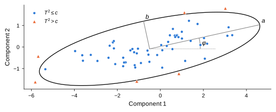
In Figure 2, the components are correlated, so the ellipse is rotated by \(\varphi =\) 12.4°, and the 6 points outside it are those flagged by Tsquared > cutoff_95pct.
With three components (pcz in hotelling_coordinates), the region is an ellipsoid, and the points are given by Equation 8 with the unit sphere \(\mathbf{e}(\theta, \psi) = (\cos\theta\sin\psi,\ \sin\theta\sin\psi,\ \cos\psi)^\top\), \(\theta \in [0, 2\pi]\), \(\psi \in [0, \pi]\), and the cutoff computed with \(k = 3\). The pts × pts points form a grid with \(\theta\) varying fastest, so each coordinate can be reshaped to (pts, pts) for surface plots.
hotelling_parameters selects the components that enter Equation 2 in one of two ways:
k, default 2). With k=2, components pcx and pcy are used and the ellipse parameters are returned. With k > 2, the first k components are used.threshold \(= \tau\)). With \(s_j^2\) the variance of column \(j\) of the scores, the proportion of variance of component \(j\) is \(s_j^2 / \sum_l s_l^2\), and \(k\) is the smallest number of leading components whose cumulative proportion reaches \(\tau\) (with a tolerance of \(\sqrt{\epsilon}\), so that \(\tau = 1\) is reachable), and at least 2. The proportions are relative to the columns of the scores passed to the function, not to the total variance of the original data.A component is treated as having near-zero variance when its proportion of variance is below rel_tol or its variance below abs_tol. If such components are among the first \(k\), they are removed with a warning, and \(k\) is recomputed on the remaining components. With k=2, a near-zero variance pcx or pcy raises an error instead. At least \(k + 2\) observations are required, so that both limits are defined.
confidence_ellipse draws the same kind of region for \(p = 2\) or 3 raw variables, optionally for each group of a categorical variable. It differs from the functions above in two ways.
robust=True, it uses the reweighted Minimum Covariance Determinant estimates computed by scikit-learn’s EllipticEnvelope with support_fraction=0.9 and random_state=42, i.e. the FAST-MCD algorithm (Rousseeuw and Van Driessen 1999) on 90% of the observations, so up to about 10% of outlying observations do not affect them. The reweighted covariance matrix is multiplied by the factor that makes it consistent at the normal distribution (Croux and Haesbroeck 1999), as by scikit-learn ≥ 1.8; pyEllipse applies this factor itself with older versions, which omit it. Without it, the variances are about 10% too small for \(p = 2\), and a 95% region contains only about 93% of a normal distribution.distribution='normal', \(c = \chi^2_{1-\alpha}(p)\), the large-sample limit, which treats the estimated mean and covariance as exact. With distribution='hotelling', \(c = \frac{p(n-1)}{n-p} F_{1-\alpha}(p, n-p)\) as in Equation 4, where \(n\) is the number of observations of the group; it is larger than the chi-square quantile, and the difference matters for small groups.At least \(p + 1\) observations (of each group) are required, so that the covariance matrix can be nonsingular and \(n - p > 0\). A singular covariance matrix, e.g. of collinear variables, gives a flat region: a line segment, or a flat ellipsoid.
from matplotlib.lines import Line2D
from pyEllipse import confidence_ellipse

population_cov = np.array([[1.0, 0.8], [0.8, 1.5]])
sizes_ce = [10, 500]
rng = np.random.default_rng(11)
samples = [
    pd.DataFrame(rng.multivariate_normal([0, 0], population_cov, size=size), columns=["x", "y"])
    for size in sizes_ce
]
regions = [
    {dist: confidence_ellipse(sample, x="x", y="y", conf_level=0.95, distribution=dist)
     for dist in ["normal", "hotelling"]}
    for sample in samples
]
c_normal = stats.chi2.ppf(0.95, 2)
area_ratio = [2 * (size - 1) / (size - 2) * stats.f.ppf(0.95, 2, size - 2) / c_normal
              for size in sizes_ce]

# Same data range for both panels
extent = max(
    max(np.abs(region[dist][["x", "y"]].to_numpy()).max() for region in regions for dist in region),
    max(np.abs(sample.to_numpy()).max() for sample in samples),
)

fig, axes = plt.subplots(1, 2, figsize=(DOUBLE, 95 * MM))
for ax, label, size, sample, region in zip(axes, "ab", sizes_ce, samples, regions):
    ax.scatter(sample["x"], sample["y"], s=14 if size < 50 else 3, color="#a6a6a6",
               linewidth=0, zorder=2)
    ax.plot(region["normal"]["x"], region["normal"]["y"], color=BLUE, lw=1.2, zorder=3)
    ax.plot(region["hotelling"]["x"], region["hotelling"]["y"], color=ORANGE, lw=1.2,
            ls="--", zorder=3)
    # Include the corners of the common range, and let the equal aspect widen x
    ax.update_datalim([(-extent, -extent), (extent, extent)])
    ax.set_aspect("equal", adjustable="datalim")
    ax.text(0.03, 0.97, f"({label})  $n$ = {size}", transform=ax.transAxes,
            ha="left", va="top")
    ax.set_xlabel("$x$")
axes[0].set_ylabel("$y$")
fig.legend(
    handles=[
        Line2D([], [], color="#a6a6a6", marker="o", ls="", markersize=4, label="Observations"),
        Line2D([], [], color=BLUE, lw=1.2, label="distribution='normal'"),
        Line2D([], [], color=ORANGE, lw=1.2, ls="--", label="distribution='hotelling'"),
    ],
    loc="outside lower center", ncols=3,
)
plt.show()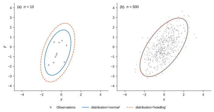
Both regions are centred on the same estimated mean and have the shape of the same estimated covariance matrix; only their size differs. As the area of the region is \(\pi c \sqrt{\det \hat{\boldsymbol{\Sigma}}}\), the Hotelling region is larger than the normal region by the ratio of the quantiles. Figure 3 shows the two regions for a small and a large sample of the same bivariate normal population: the Hotelling region is 1.67 times larger in area with \(n =\) 10, and 1.008 times larger with \(n =\) 500.
With \(\hat{\boldsymbol{\Sigma}} = \mathbf{V}\boldsymbol{\Lambda}\mathbf{V}^\top\), the points are \(\hat{\boldsymbol{\mu}} + \mathbf{V}(c\boldsymbol{\Lambda})^{1/2}\mathbf{e}\), with 361 values of \(\theta\) (one per degree) for an ellipse and a 50 × 50 grid for an ellipsoid. This is the same set of boundary points as Equation 8, parametrized along the eigenvectors.