Outlier detection with PCA scores

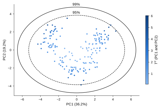
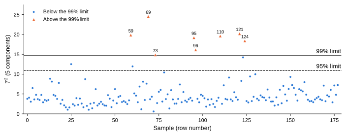
Score plot with Hotelling’s ellipses, T-squared control chart, and the contribution of each component to the flagged samples.

This example fits a PCA model to the wine data and looks for unusual samples among the samples the model was fitted on. All the numbers in the text are computed when this page is built, and the figures are ready for publication (see Saving the figures).

Data and PCA model

The wine data has 178 samples and 13 chemical measurements. The measurements are standardized, since they have different units, and all principal components are kept.

import numpy as np
import pandas as pd
from matplotlib.colors import LinearSegmentedColormap
from sklearn.datasets import load_wine
from sklearn.decomposition import PCA
from sklearn.preprocessing import StandardScaler

from pyEllipse import hotelling_coordinates, hotelling_parameters

X = StandardScaler().fit_transform(load_wine().data)
pca = PCA().fit(X)
scores = pca.transform(X)
explained = pca.explained_variance_ratio_

pd.DataFrame(
    {"Explained variance": explained, "Cumulative": np.cumsum(explained)},
    index=[f"PC{j}" for j in range(1, len(explained) + 1)],
).head(6).style.format("{:.1%}")

	Explained variance	Cumulative
PC1	36.2%	36.2%
PC2	19.2%	55.4%
PC3	11.1%	66.5%
PC4	7.1%	73.6%
PC5	6.6%	80.2%
PC6	4.9%	85.1%

The scores are the samples the model was fitted on, so the exact limit of T-squared for them is the Beta limit, method="beta" (see Control limits).

Figure style

The figures are sized for journal columns (89, 140 or 183 mm wide), with 8–9 pt text at the printed size, colours that remain distinct with colour-vision deficiencies, and line styles or marker shapes that keep them readable in grayscale.

import matplotlib.pyplot as plt
from cycler import cycler

# Figure widths of most journals, in inches: single, 1.5 and double column
MM = 1 / 25.4
SINGLE, ONE_HALF, DOUBLE = 89 * MM, 140 * MM, 183 * MM

# Colour-blind-safe colours, used in this order; each figure also varies line style
# or marker shape, so it can be printed in grayscale
BLUE, ORANGE, AQUA, GREY = "#2a78d6", "#eb6834", "#1baf7a", "#808080"

plt.rcParams.update({
    # Text and mathematics in the same sans-serif font, at the printed size
    "font.family": "sans-serif",
    "font.sans-serif": ["Arial", "Helvetica", "Liberation Sans", "DejaVu Sans"],
    "font.size": 9,
    "axes.labelsize": 9,
    "xtick.labelsize": 8,
    "ytick.labelsize": 8,
    "legend.fontsize": 8,
    "mathtext.fontset": "custom",
    "mathtext.rm": "sans",
    "mathtext.it": "sans:italic",
    "mathtext.bf": "sans:bold",
    "mathtext.sf": "sans",
    "mathtext.cal": "sans:italic",
    # Thin black axes, outward ticks, no grid
    "axes.edgecolor": "black",
    "axes.linewidth": 0.6,
    "axes.spines.top": False,
    "axes.spines.right": False,
    "axes.prop_cycle": cycler(color=[BLUE, ORANGE, AQUA]),
    "xtick.major.width": 0.6,
    "ytick.major.width": 0.6,
    "xtick.major.size": 3,
    "ytick.major.size": 3,
    "xtick.direction": "out",
    "ytick.direction": "out",
    "lines.linewidth": 1.2,
    "legend.frameon": False,
    # Saved figures keep the exact size set with figsize
    "figure.constrained_layout.use": True,
    # Vector output with embedded TrueType fonts; 600 dpi for raster formats
    "pdf.fonttype": 42,
    "ps.fonttype": 42,
    "svg.fonttype": "none",
    "savefig.dpi": 600,
})

Score plot with Hotelling’s ellipses

hotelling_parameters computes T-squared on the first two components and its cutoffs, and hotelling_coordinates the points of the matching ellipses.

res_2 = hotelling_parameters(scores, pcx=1, pcy=2, method="beta")
ellipse_95 = hotelling_coordinates(scores, pcx=1, pcy=2, conf_limit=0.95, method="beta")
ellipse_99 = hotelling_coordinates(scores, pcx=1, pcy=2, conf_limit=0.99, method="beta")

t2_2 = res_2["Tsquared"]["value"]
above_95 = np.flatnonzero(t2_2 > res_2["cutoff_95pct"])
res_2["Ellipse"].round(3)

	a_99pct	b_99pct	a_95pct	b_95pct	angle
0	6.535	4.76	5.295	3.857	0.0

# Sequential colour map, light to dark, for the magnitude of T-squared
t2_cmap = LinearSegmentedColormap.from_list(
    "t2", ["#86b6ef", "#5598e7", "#2a78d6", "#1c5cab", "#104281"]
)

fig, ax = plt.subplots(figsize=(ONE_HALF, 94 * MM))
points = ax.scatter(scores[:, 0], scores[:, 1], c=t2_2, cmap=t2_cmap, s=12,
                    edgecolor="white", linewidth=0.3, zorder=3)
for ellipse, label, style in [(ellipse_95, "95%", "--"), (ellipse_99, "99%", "-")]:
    ax.plot(ellipse["x"], ellipse["y"], color="black", lw=0.9, ls=style)
    top = ellipse["y"].idxmax()
    ax.annotate(label, (ellipse["x"][top], ellipse["y"][top]), xytext=(0, 2),
                textcoords="offset points", ha="center", va="bottom")
fig.colorbar(points, ax=ax, label=r"$T^2$ (PC1 and PC2)", shrink=0.75, aspect=25)
ax.set_aspect("equal", adjustable="datalim")
ax.set_xlabel(f"PC1 ({explained[0]:.1%})")
ax.set_ylabel(f"PC2 ({explained[1]:.1%})")
plt.show()

Figure 1: Scores on the first two principal components, coloured by their T-squared value on these components, with the 95% (dashed) and 99% (solid) Hotelling’s ellipses (Beta limits).

The scores are uncorrelated, so the ellipses are aligned with the axes (angle is 0). On these two components, 2 samples lie outside the 95% ellipse (rows 3, 115), and none outside the 99% ellipse.

T-squared on more components

Two components explain only 55% of the variance. With threshold=0.8, hotelling_parameters uses the smallest number of components that explain at least 80% of it.

res = hotelling_parameters(scores, threshold=0.8, method="beta")
k = res["nb_comp"]
t2 = res["Tsquared"]["value"]
flagged = np.flatnonzero(t2 > res["cutoff_99pct"])
print(f"{k} components, 95% limit {res['cutoff_95pct']:.2f}, 99% limit {res['cutoff_99pct']:.2f}")
print("Rows above the 99% limit:", flagged.tolist())

5 components, 95% limit 10.88, 99% limit 14.66
Rows above the 99% limit: [59, 69, 73, 95, 96, 110, 121, 124]

rows = np.arange(len(t2))
above = t2.to_numpy() > res["cutoff_99pct"]

fig, ax = plt.subplots(figsize=(DOUBLE, 70 * MM))
for level, style in [("95", "--"), ("99", "-")]:
    cutoff = res[f"cutoff_{level}pct"]
    ax.axhline(cutoff, color="black", lw=0.8, ls=style)
    ax.annotate(f"{level}% limit", (1, cutoff), xycoords=("axes fraction", "data"),
                xytext=(0, 2), textcoords="offset points", ha="right", va="bottom")
ax.scatter(rows[~above], t2[~above], s=10, marker="o", color=BLUE, edgecolor="white",
           linewidth=0.3, label="Below the 99% limit", zorder=3)
ax.scatter(rows[above], t2[above], s=20, marker="^", color=ORANGE, edgecolor="white",
           linewidth=0.3, label="Above the 99% limit", zorder=3)
for row in rows[above]:
    ax.annotate(str(row), (row, t2[row]), xytext=(0, 4), textcoords="offset points",
                ha="center", fontsize=7)
ax.set_xlim(-2, len(t2) + 1)
ax.set_ylim(0, 1.12 * t2.max())
ax.set_xlabel("Sample (row number)")
ax.set_ylabel(f"$T^2$ ({k} components)")
ax.legend(loc="upper left")
plt.show()

Figure 2: T-squared of each sample on the components that explain 80% of the variance, with the 95% (dashed) and 99% (solid) Beta limits. The samples above the 99% limit (triangles) are labelled with their row number.

Which components make a sample unusual?

For uncorrelated scores, T-squared is a sum of one term per component, \(t_{ij}^2 / s_j^2\) (see Uncorrelated scores). These contributions show which components make each flagged sample unusual; their sum is the T-squared value returned by hotelling_parameters.

components = [f"PC{j}" for j in range(1, k + 1)]
contributions = pd.DataFrame(
    scores[:, :k] ** 2 / scores[:, :k].var(axis=0, ddof=1), columns=components
)
assert np.allclose(contributions.sum(axis=1), t2)  # the contributions add up to T-squared

table = contributions.loc[flagged].assign(**{"T²": t2[flagged]})
table.index.name = "Row"
(
    table.style.format("{:.2f}")
    .highlight_max(axis=1, subset=components, props="font-weight: bold")
)

Table 1: Contribution of each component to the T-squared value of the samples above the 99% limit. The largest contribution of each sample is in bold.

	PC1	PC2	PC3	PC4	PC5	T²
Row
59	0.18	3.76	14.46	1.20	0.24	19.84
69	0.82	0.78	1.05	1.44	20.43	24.53
73	1.39	0.03	7.83	1.04	4.57	14.85
95	1.37	0.01	0.43	1.15	16.22	19.18
96	0.06	0.05	1.18	1.77	13.05	16.12
110	0.43	0.80	0.01	12.73	5.62	19.60
121	0.38	0.03	19.65	0.06	0.07	20.18
124	0.20	0.83	1.51	15.55	0.29	18.38

F or Beta limit?

The default method="f" gives larger limits than method="beta"; for the samples the model was fitted on, it is conservative, so it can miss samples that the exact Beta limit flags.

summary = []
for method in ["beta", "f"]:
    r = hotelling_parameters(scores, threshold=0.8, method=method)
    for level in ["95", "99"]:
        cutoff = r[f"cutoff_{level}pct"]
        summary.append({"Method": method, "Level": f"{level}%", "Limit": cutoff,
                        "Samples above": int((r["Tsquared"]["value"] > cutoff).sum())})
pd.DataFrame(summary).style.hide(axis="index").format({"Limit": "{:.2f}"})

Table 2: Limits of T-squared on the components that explain 80% of the variance, and number of samples above them, by method and confidence level.

Method	Level	Limit	Samples above
beta	95%	10.88	11
beta	99%	14.66	8
f	95%	11.59	11
f	99%	15.98	7

With 178 samples, the two limits are close; for small data sets, the difference is much larger (see the figure of the limits on the Theory page).

Saving the figures

With the figure style above, figures keep the size set with figsize when saved, and their fonts are embedded as TrueType, as journals require. Save each figure in the format your journal asks for:

fig.savefig("score-plot.pdf")             # vector, accepted by most journals
fig.savefig("score-plot.eps")             # vector, for journals that require EPS
fig.savefig("score-plot.tiff", dpi=600)   # raster, for journals that require TIFF