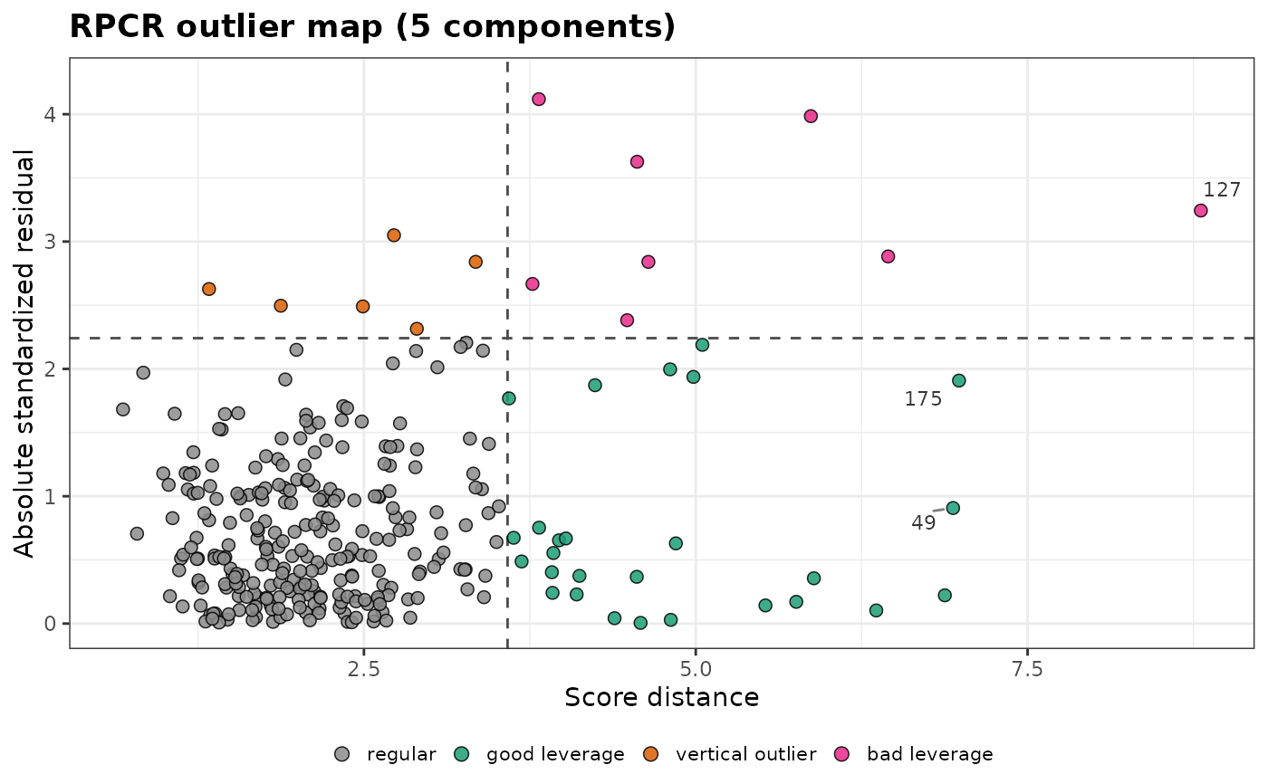
Robust Principal Component Regression (RPCR)

Robust principal component regression by the RPCR method of Hubert and Verboven (2003): the robust principal components of the predictors (robpca()), followed by a robust regression of the responses on the scores. Outlying spectra and wrong reference values have little influence on the model, and the regression outlier map (plot_outlier_map()) classifies them.

Usage

rpcr(x, y, ncomp, kmax = 10, alpha = 0.75, ndir = 250, nsamp = 500)

Arguments

x: A numeric matrix or data frame of the predictors (spectra), one observation per row.
y: A numeric vector, matrix or data frame of the responses, with one row per observation.
ncomp: The number of components of the model.
kmax: The largest number of components considered: the number of components of the robust PCA, so the model also depends on kmax (see Details). Default is 10; it is raised to ncomp if needed, and lowered when there are too few observations or variables.
alpha: The fraction of observations assumed to be regular, between 0.5 and 1, for robpca() and the robust regression. Default is 0.75.
ndir: The number of random directions of the outlyingness in robpca(). Default is 250.
nsamp: The number of random subsets of FAST-MCD in robpca(), and of the LTS or MCD regression. Default is 500.

Value

An object of class specproc_rpcr, a list with:

coefficients, intercept: the regression coefficients (a \(p \times q\) matrix) and intercepts.
x_loadings, x_scores, eigenvalues: the loadings \(P\), scores \(T\) and eigenvalues of the ncomp components.
y_loadings: the slopes \(A\) of the regression of the responses on the scores (ncomp rows).
center: the robust center of the predictors.
fitted, residuals: the fitted values and residuals.
sigma: the robust covariance matrix of the residuals.
sd, rd, od: the score, residual and orthogonal distances of each observation, and cutoff_sd, cutoff_rd, cutoff_od their cut-offs.
R2: the robust \(R^2\) of the model (see Details).
outlier_type: a factor classifying each observation as "regular", "good leverage", "vertical outlier" or "bad leverage".
weights: 1 for the observations of the final (reweighted) regression, 0 for the others.
components: a tibble with the robust R2 and RMSE of the models with 1 to kmax components.
models: the coefficients and intercept of the models with 1 to kmax components, for predictions with another number of components (predict(fit, newdata, ncomp = )).
ncomp, kmax, h, alpha: the settings used, and regression, "LTS" or "MCD".

Use predict() for the predictions of new observations.

Details

The method has two steps:

Robust PCA. robpca() is applied to the predictors with kmax components. It gives a robust center \(\hat\mu_x\), the loadings \(P\) and the eigenvalues \(l_a\), and the scores \(t_i = P^T (x_i - \hat\mu_x)\).
Robust regression. The responses are regressed on the first ncomp scores. With one response, this is the reweighted least trimmed squares (LTS) regression of robustbase::ltsReg(). With several responses, it is the MCD regression of Rousseeuw, Van Aelst, Van Driessen and Agullo (2004): least squares from the reweighted MCD of the scores and responses, then least squares on the observations whose residual distance is below \(\sqrt{\chi^2_{q, 0.99}}\).

The regression coefficients are \(B = P_k A_k\), from the loadings \(P_k\) and the slopes \(A_k\) of the regression on the first ncomp scores.

Diagnostics. As for rsimpls(): the score distance \(SD_i = \sqrt{\sum_a t_{ia}^2 / l_a}\) has the cut-off \(\sqrt{\chi^2_{k, 0.975}}\), the residual distance (with one response, the absolute standardized residual) the cut-off \(\sqrt{\chi^2_{q, 0.975}}\), and the orthogonal distance \(OD_i = \|x_i - \hat\mu_x - P t_i\|\) the cut-off of robpca(). Observations beyond the score cut-off only are good leverage points, beyond the residual cut-off only vertical outliers, and beyond both bad leverage points. The robust \(R^2\) of the model (R2) is computed on the observations whose orthogonal and residual distances are both below their cut-offs.

Number of components. components gives, for 1 to kmax components, the robust \(R^2\) and root mean squared error on the observations that are regular in every one of these models; use robust_rmsecv() for the robust cross-validated error. These models all come from the same robust PCA, with kmax components, of which they use the first ncomp, so the model also depends on kmax. With kmax = ncomp, the robust PCA has ncomp components, as in the paper.

Differences from the paper.

The models with fewer components than kmax use the first components of the robust PCA with kmax components (see above).
The residual covariance of the MCD regression is multiplied by the consistency factor \(0.99 / P(\chi^2_{q+2} \le \chi^2_{q, 0.99})\), as the observations beyond the cut-off are left out.

This is an independent implementation of the published description. robpca(), the LTS and the MCD use random subsets, so use set.seed() for reproducible results.

References

Hubert, M., Verboven, S. (2003). A robust PCR method for high-dimensional regressors. Journal of Chemometrics, 17(8-9):438-452.
Rousseeuw, P.J., Van Aelst, S., Van Driessen, K., Agullo, J. (2004). Robust multivariate regression. Technometrics, 46(3):293-305.
Hubert, M., Rousseeuw, P.J., Vanden Branden, K. (2005). ROBPCA: a new approach to robust principal component analysis. Technometrics, 47(1):64-79.

Author

Christian L. Goueguel

Examples

data(forageLIBS)
wl <- suppressWarnings(as.numeric(names(forageLIBS)))
spectra <- forageLIBS[which(wl > 380 & wl < 430)]  # Ca II and Ca I lines
cal <- 1:300
set.seed(1)
fit <- rpcr(spectra[cal, ], forageLIBS$Ca[cal], ncomp = 5)
fit
#> Robust PCR (RPCR, LTS regression)
#> 
#> Observations:   300 (h = 225)
#> Variables:      594
#> Responses:      1
#> Components:     5 (robust R2 of 1 to 10 components: 0.152 0.191 0.203 0.578 0.580 0.603 0.701 0.725 0.729 0.743)
#> Robust R2:      0.532
#> Residual scale: 0.1238
#> 
#> Outlier types:
#> 
#>          regular    good leverage vertical outlier     bad leverage 
#>              259               27                6                8 
#> 
#> Orthogonal outliers: 71
head(predict(fit, spectra[-cal, ]))
#> [1] 0.4693860 0.3976267 0.6559014 0.5791613 0.7150952 0.3257995
plot_outlier_map(fit)