Plot a Self-Organizing Map

Draws a map fitted by som(): the number of spectra per unit, the distances between neighboring prototypes, the component planes, the spectra on the map, or the prototype spectra.

Usage

plot_som(
  object,
  type = c("counts", "umatrix", "quality", "component", "mapping", "prototypes"),
  variables = NULL,
  colour = NULL,
  newdata = NULL,
  units = NULL,
  title = NULL
)

Arguments

object

A map fitted by som().

type

The plot: "counts" (default), "umatrix", "quality", "component", "mapping" or "prototypes".

variables

For "component": the variables, as wavelengths (the nearest channel is used) or column names.

colour

For "mapping": a vector with one value per training spectrum, such as a concentration or a class.

newdata

For "mapping": optional new spectra to place on the map.

units

For "prototypes": the units whose prototypes are drawn.

title

The plot title.

Value

A ggplot object.

Details

The types of plot are:

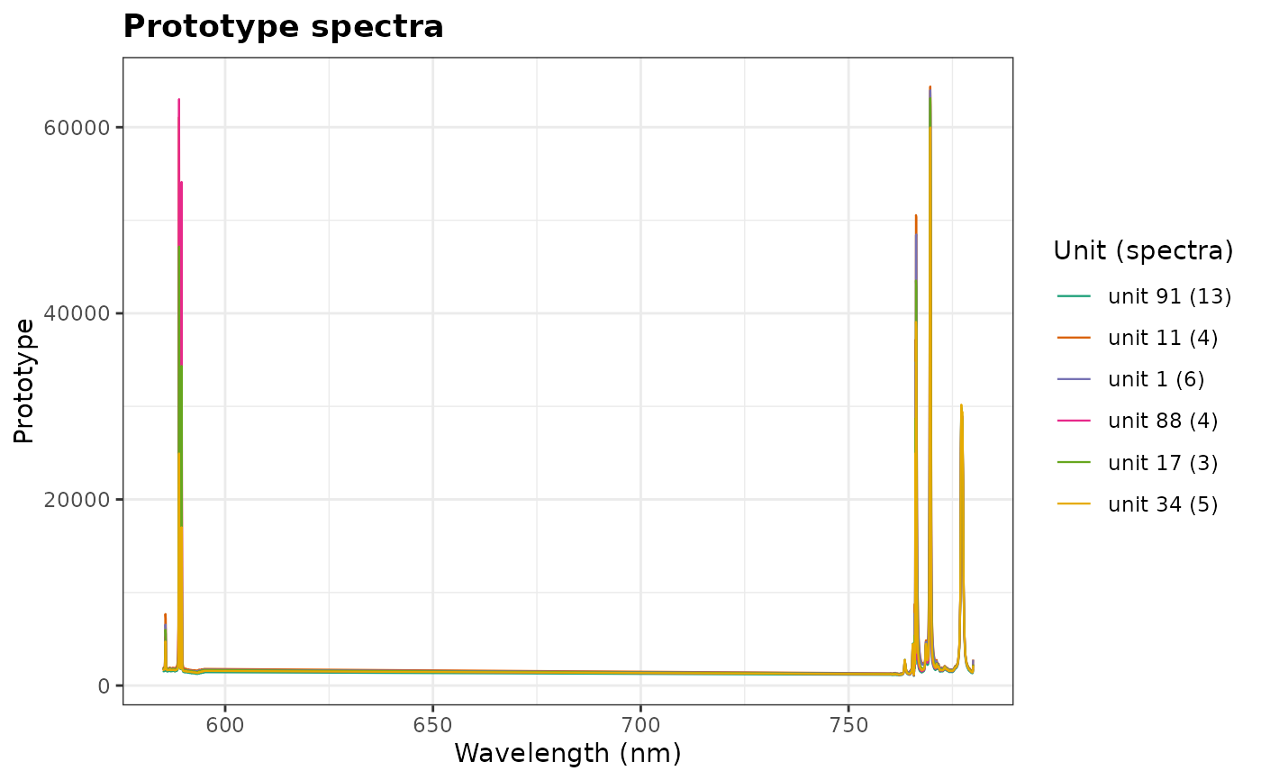
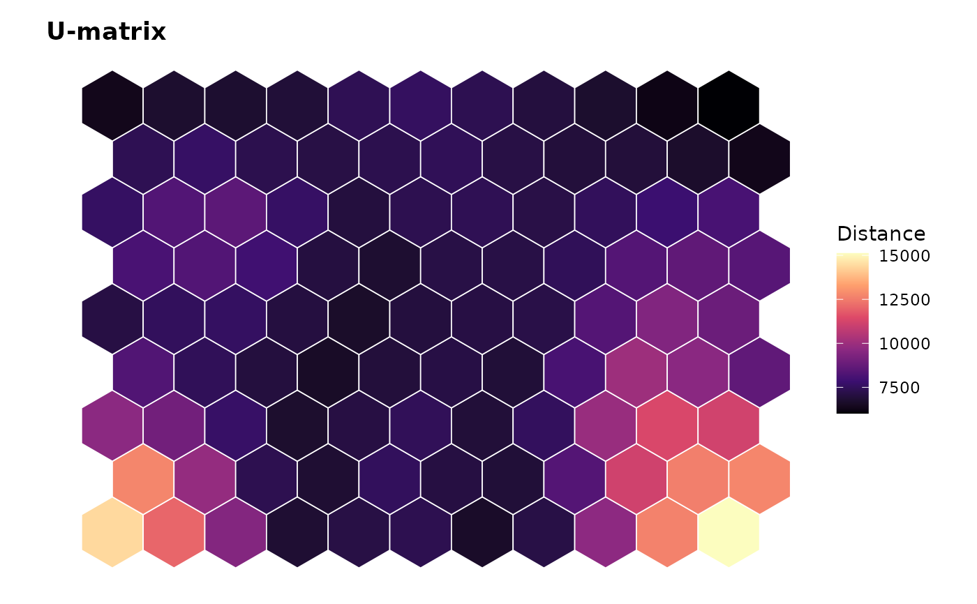
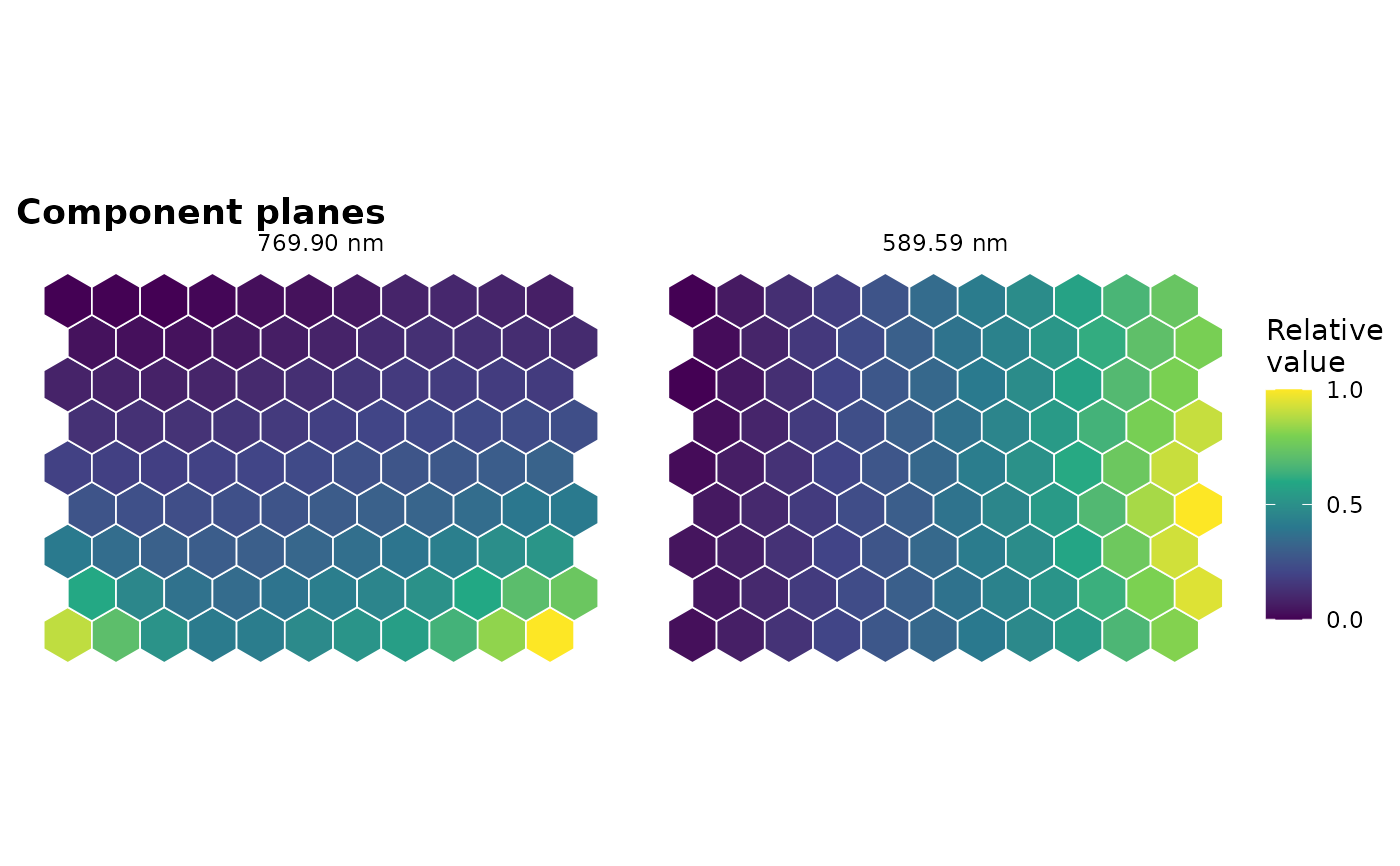
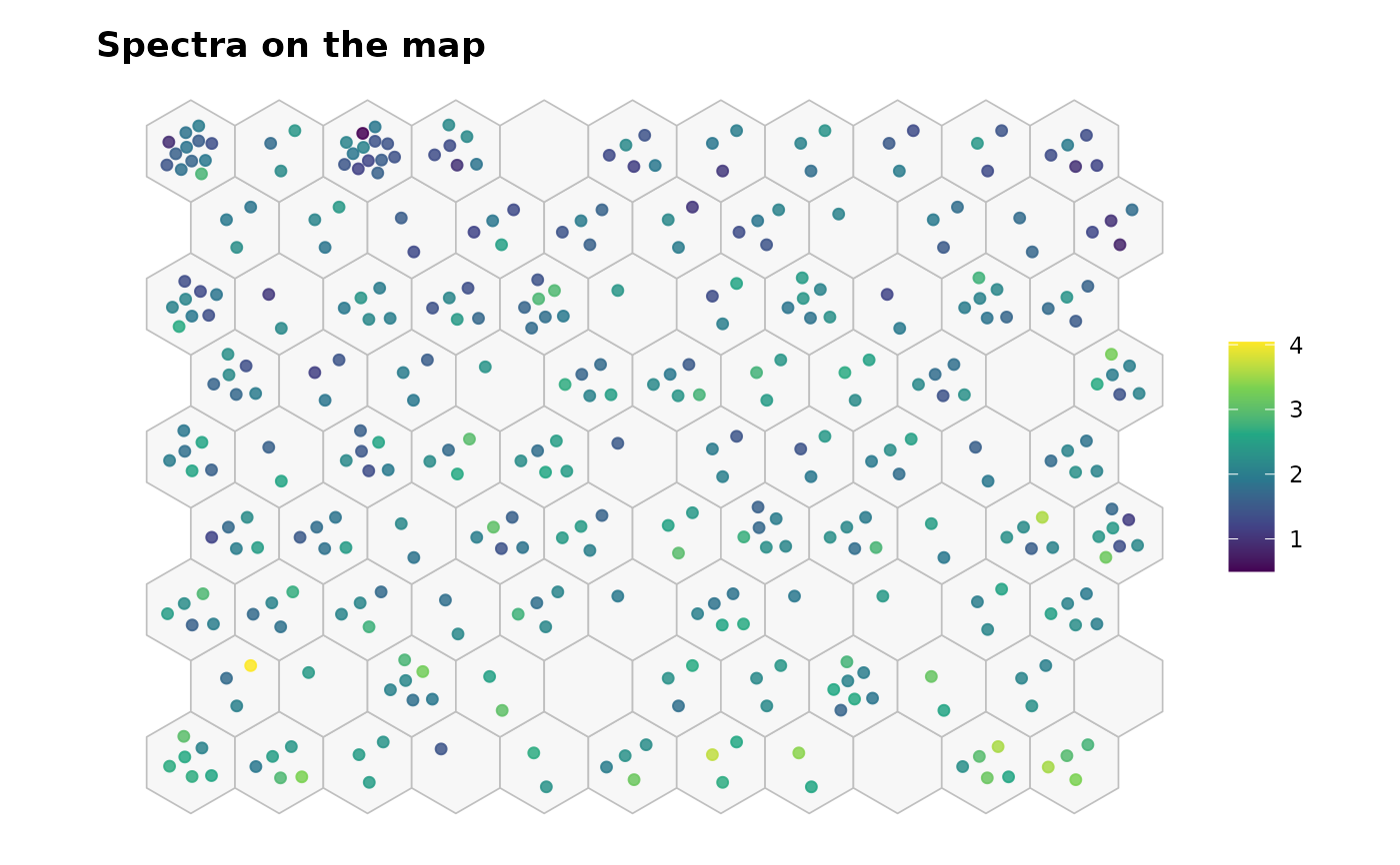
• "counts": the number of training spectra on each unit (empty units in white).

• "umatrix": the unified distance matrix, the mean distance of each prototype to those of its neighbors: high values (light) are the boundaries between groups of similar spectra, low values (dark) the groups themselves.

• "quality": the mean quantization error of the spectra of each unit.

• "component": the component planes, the value of the prototypes at each of the variables (one panel per variable): which units have intense emission lines. Each plane is scaled from its lowest (0) to its highest (1) unit, so that weak lines are as readable as strong ones.

• "mapping": the training spectra on their units (spread within the unit), colored by colour, and, with newdata, the new spectra as triangles, the novel ones circled in red.

• "prototypes": the prototype spectra of the units against wavelength. By default, six prototypes spread over the map: the unit with the most spectra, then, in turn, the unit whose prototype is the farthest from those already chosen.

See also

som(), predict.specproc_som()

Examples

data(forageLIBS)
# the Na I and K I resonance lines
wl <- suppressWarnings(as.numeric(names(forageLIBS)))
spectra <- forageLIBS[which((wl > 585 & wl < 595) | (wl > 760 & wl < 780))]
fit <- som(spectra)
plot_som(fit, type = "umatrix")

# component planes of the K I and Na I lines
plot_som(fit, type = "component", variables = c(769.90, 589.59))

plot_som(fit, type = "mapping", colour = forageLIBS$K)

plot_som(fit, type = "prototypes")