Plots of the Laser Shots and of their Rejection

Shows the shots of a LIBS data set and the shots rejected by reject_shots(): their criteria, their spectra, the trends along the shots, and the samples, to judge the rejection before averaging the shots.

Usage

plot_shots(
  x,
  type = c("heatmap", "criteria", "spectra", "order", "samples"),
  sample = NULL,
  wavelength = NULL,
  label = 10,
  acquisition = NULL,
  arrange = c("data", "extreme"),
  smooth = NULL,
  plot = TRUE,
  title = NULL,
  caption = TRUE,
  base_size = 11
)

Arguments

x: The result of reject_shots() (with drop = FALSE).
type: The view: "heatmap" (default), "criteria", "spectra", "order" or "samples" (see Details).
sample: For type = "spectra", the sample to draw: a value of the sample column. Default is the sample with the most rejected shots.
wavelength: For type = "spectra", an optional wavelength range (nm) to zoom on.
label: For type = "criteria", the number of rejected shots labeled, the most extreme first. Default is 10; 0 for none.
acquisition: For type = "heatmap", an optional column of x (unquoted or as a string) giving the order of the measurements, such as the measurement number or the acquisition time: the rows follow it.
arrange: For type = "heatmap" without acquisition, the order of the rows: "data" (default), that of the samples in x, or "extreme", the samples with the most extreme shots first.
smooth: For type = "heatmap", an odd number k of consecutive measurements: each cell is the running median of the z-scores of that shot number over them. Needs acquisition. Default is NULL, no smoothing.
plot: A logical: plot (TRUE, default) or return the table of the view (the shots with their z-scores, smoothed or not, the shots of the sample, the shot numbers or the samples).
title: The plot title. A long title is split into a title and a subtitle.
caption: TRUE (default), a caption saying how to read the plot, with the number of rejected shots; FALSE, no caption; or a caption of your own.
base_size: The size of the text, in points. Default is 11.

Value

A ggplot (or patchwork) object, or with plot = FALSE a tibble.

Details

Five views of the result of reject_shots():

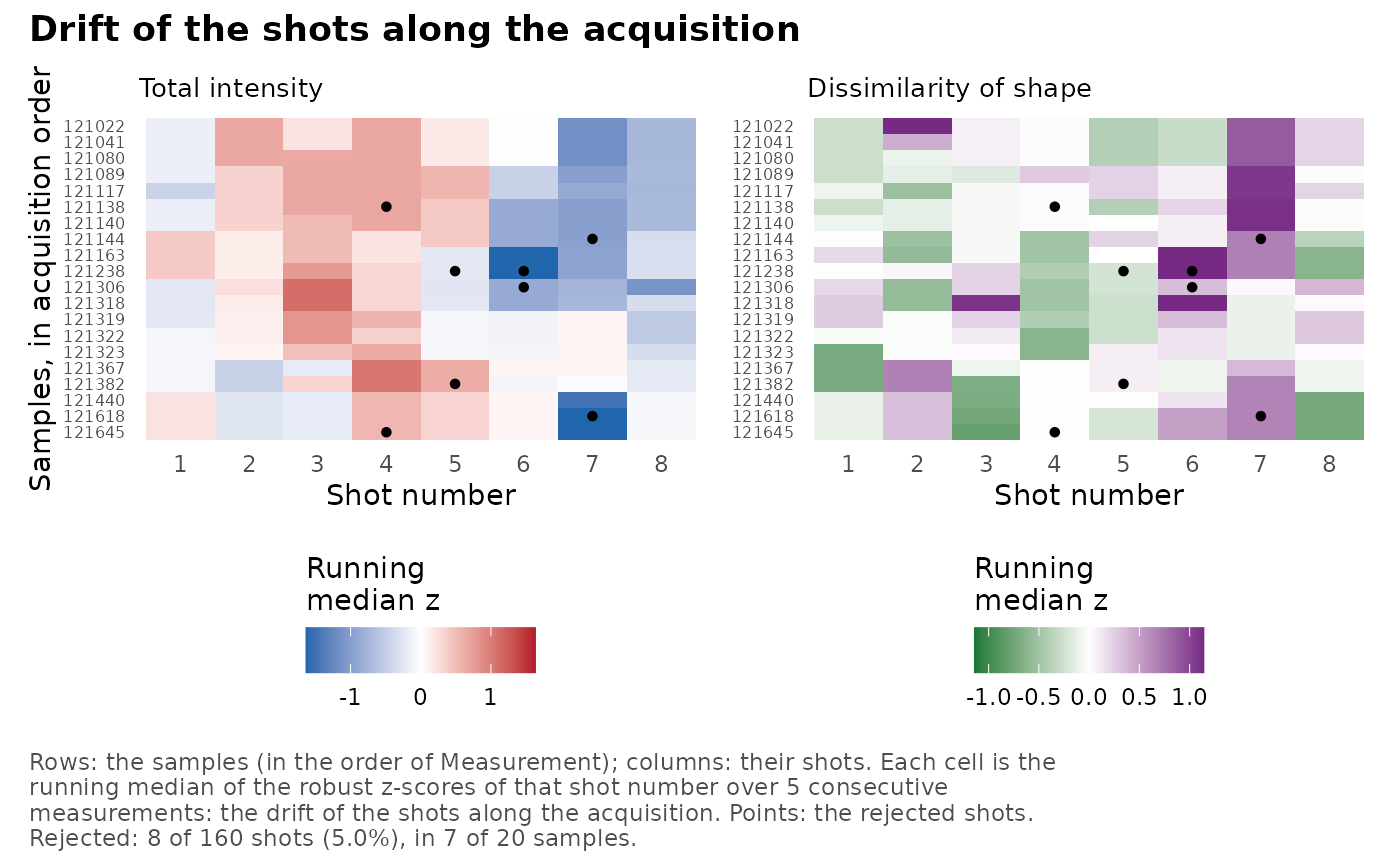
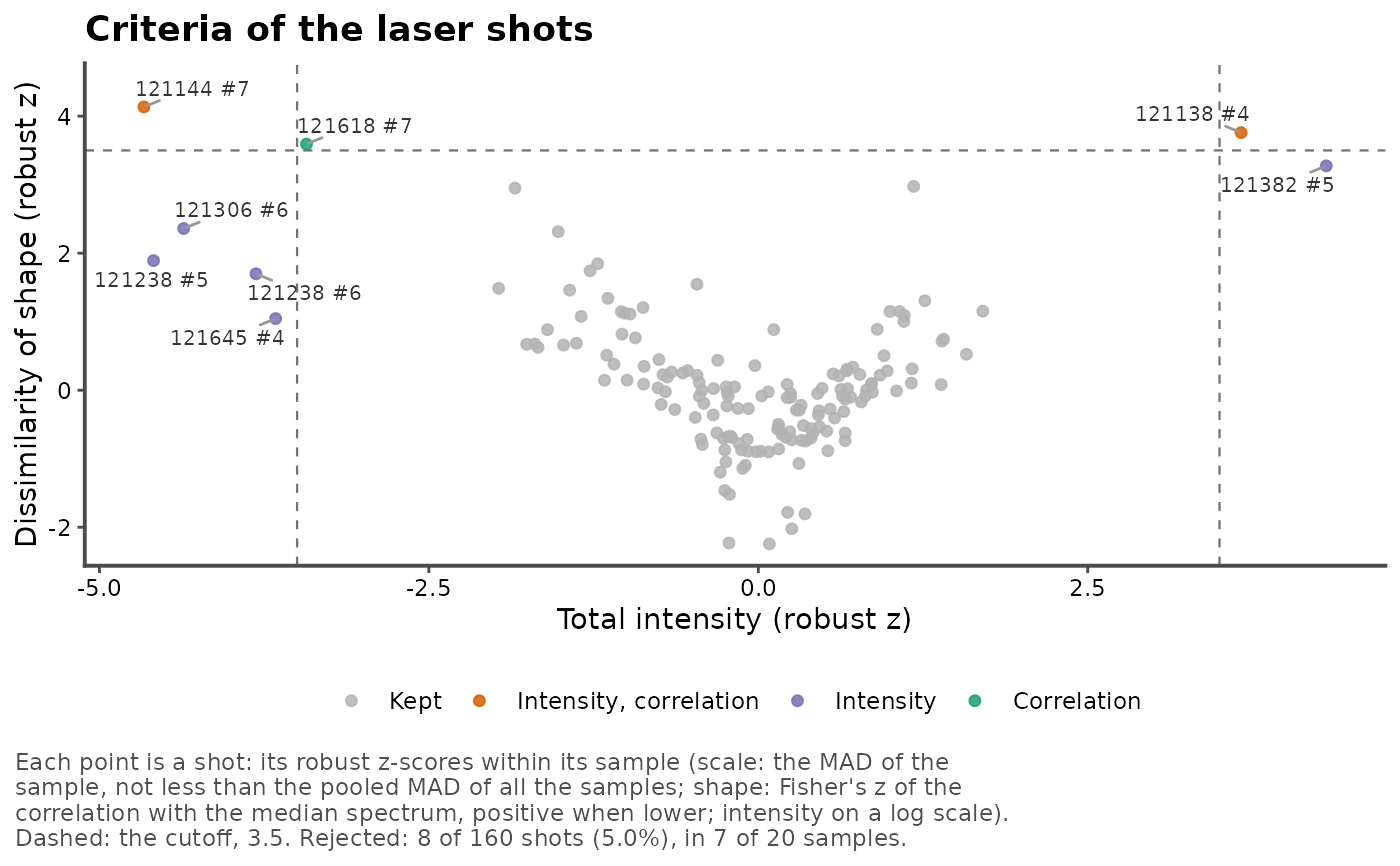
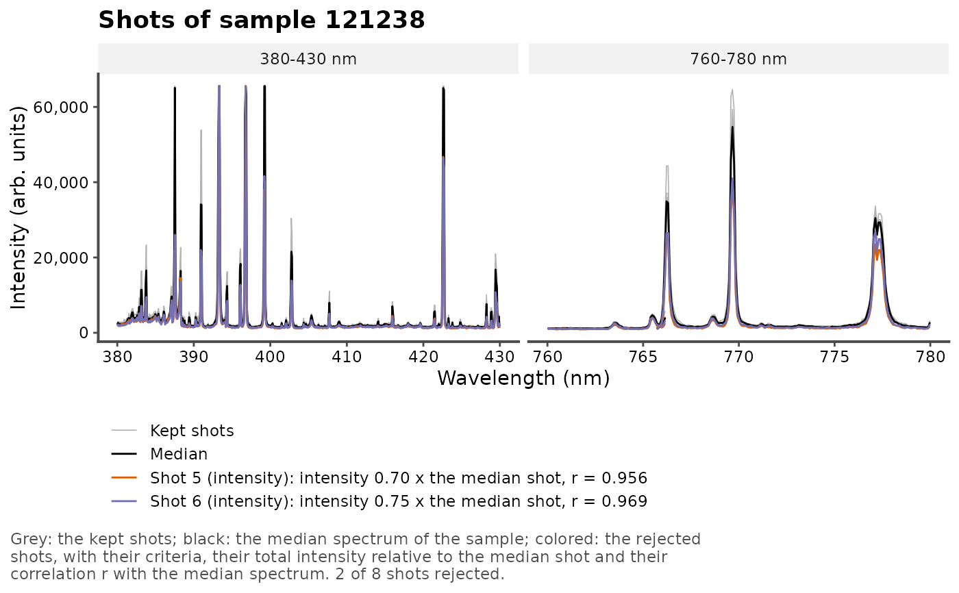
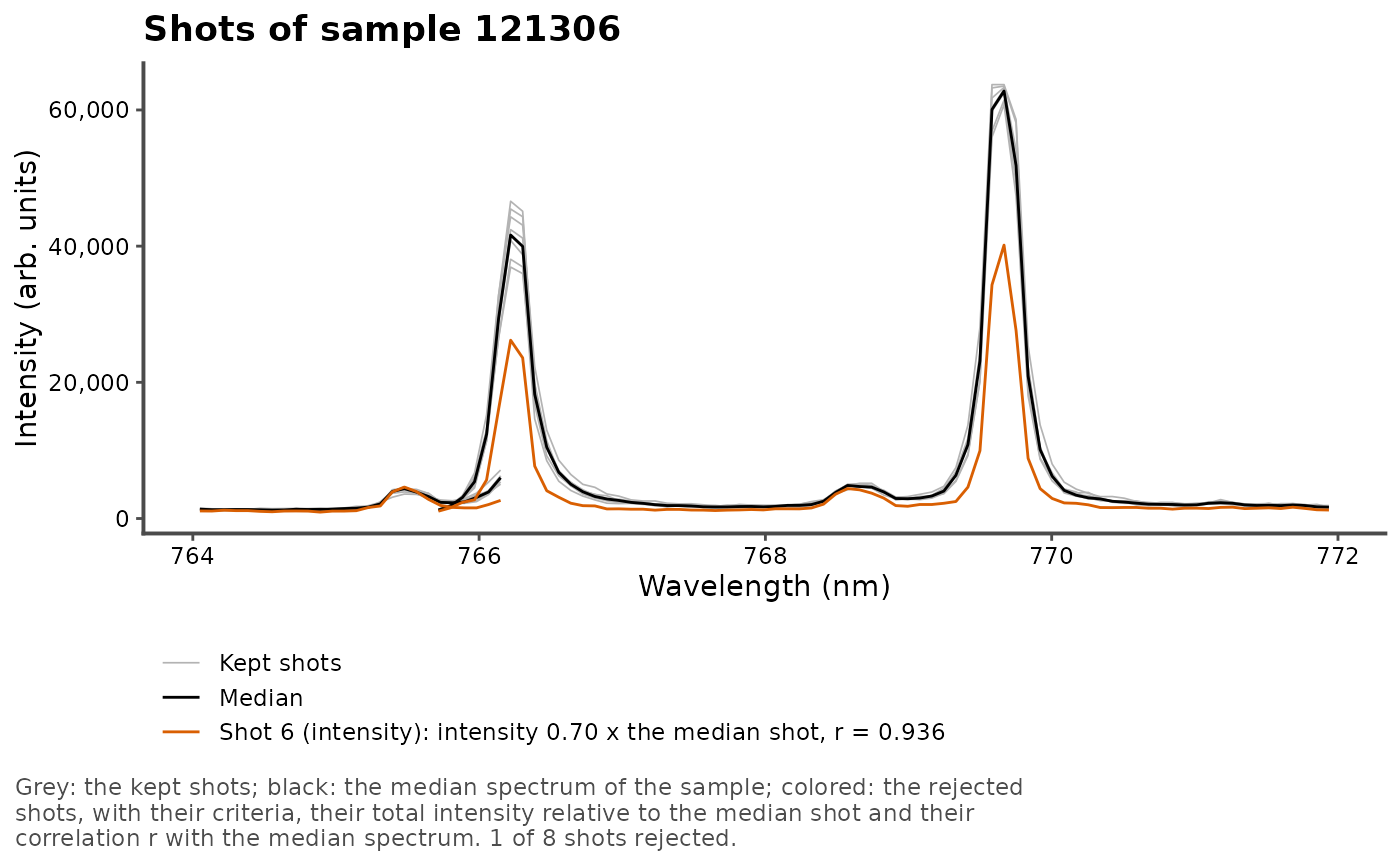
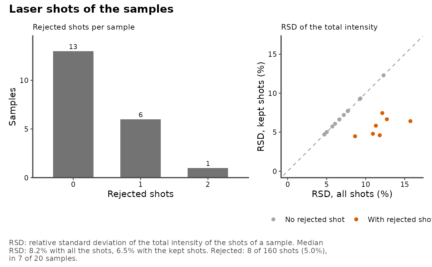
"heatmap" (default): a map of the samples (rows) by the shot number (columns), one panel per criterion, colored by the robust z-score of each shot: white below 1 (the ordinary variability of the shots), then in steps up to the cutoff and beyond it, the rejected shots outlined. It shows at a glance the rejected shots, the samples whose shots vary (rows), consecutive rejected shots (a problem of focus or surface rather than a misfire), and the trends along the shot number (columns). With acquisition, the rows follow the order of the measurements; arrange = "extreme" puts the samples with the most extreme shots first. With smooth = k (and acquisition), each cell is the running median of the z-scores of that shot number over k consecutive measurements, the rejected shots as points: the drift of the shots along the acquisition (laser energy, fouling of the optics), when the trend along the shot number changes from one period to another. Without the acquisition order, neighboring rows are unrelated samples, and smoothing them would invent patterns.
"criteria": the robust z-scores of the shots (total intensity against the dissimilarity of shape, or the criteria used), with the cutoff: the rejected shots are colored by their criteria, and the most extreme labeled (sample and shot). Shots just beyond the cutoff are borderline; a gap between the rejected shots and the others shows clear outliers.
"spectra": the shots of one sample (sample, by default the sample with the most rejected shots): the kept shots in grey, the median spectrum in black, and each rejected shot in color, with its criteria, its total intensity relative to the median shot and its correlation with the median spectrum. wavelength zooms on a range.
"order": along the shot number, the total intensity of the shots relative to their sample, their dissimilarity of shape to the median spectrum of their sample (\(1 - r\), on a log scale) and the share of rejected shots. A trend shows the first shots on the surface of the sample (cleaning shots) or the drift of the ablation in its crater, which the rejection, made within each sample, does not correct: discard the first shots, or check that the trend is the same for all samples.
"samples": the number of samples by their number of rejected shots, and the relative standard deviation (RSD) of the total intensity of the shots of each sample, with all its shots and with the kept ones: the gain of precision of the rejection, and the samples whose shots vary most (heterogeneous samples, or a poor laser focus).

The shot numbers are the .shot column of reject_shots() (its shot argument, or the order of the rows in each sample).

Author

Christian L. Goueguel

Examples

data(forageShots)
res <- reject_shots(forageShots, Measurement, shot = shot)
if (rlang::is_installed("patchwork")) {
  # the samples by the shot number, in the order of the measurements
  plot_shots(res, acquisition = Measurement)
  # the drift of the shots along the acquisition: running medians over 5
  # consecutive measurements
  plot_shots(res, acquisition = Measurement, smooth = 5)
}

# the criteria of the shots, the rejected ones labeled
plot_shots(res, type = "criteria")

# the shots of the sample with the most rejected shots
plot_shots(res, type = "spectra")

# a zoom on the K I lines
plot_shots(res, type = "spectra", sample = 121306, wavelength = c(764, 772))

# \donttest{
if (rlang::is_installed("patchwork")) {
  # the trends along the shots, and the precision of the samples
  plot_shots(res, type = "order")
  plot_shots(res, type = "samples")
}

# }
# the table of the samples
plot_shots(res, type = "samples", plot = FALSE)
#> # A tibble: 20 × 5
#>    Measurement     n n_rejected rsd_all rsd_kept
#>    <chr>       <int>      <int>   <dbl>    <dbl>
#>  1 121022          8          0    4.70     4.70
#>  2 121041          8          0    6.08     6.08
#>  3 121080          8          0    9.25     9.25
#>  4 121089          8          0    7.70     7.70
#>  5 121117          8          0    7.20     7.20
#>  6 121138          8          1   10.9      4.80
#>  7 121140          8          0    5.02     5.02
#>  8 121144          8          1   11.3      5.83
#>  9 121163          8          0   12.3     12.3 
#> 10 121238          8          2   15.7      6.42
#> 11 121306          8          1   12.7      6.66
#> 12 121318          8          0    4.76     4.76
#> 13 121319          8          0    6.63     6.63
#> 14 121322          8          0    5.73     5.73
#> 15 121323          8          0    7.74     7.74
#> 16 121367          8          0    9.33     9.33
#> 17 121382          8          1   11.8      4.61
#> 18 121440          8          0    6.65     6.65
#> 19 121618          8          1    8.65     4.47
#> 20 121645          8          1   12.1      7.46