Plot a Two-Dimensional Embedding

Draws the samples in two dimensions of an embedding, such as UMAP coordinates from embed::step_umap(), principal component scores from recipes::step_pca(), robpca() or stats::prcomp(), colored by a variable.

Usage

plot_embedding(
  data,
  x = NULL,
  y = NULL,
  colour = NULL,
  size = 2,
  alpha = 0.8,
  ellipse = FALSE,
  conf_level = 0.975,
  robust = FALSE,
  distribution = "normal",
  hotelling = "none",
  k = 2,
  t2_method = "f",
  flag = FALSE,
  label = NULL,
  biplot = FALSE,
  biplot_top = 10,
  aspect_ratio = 0.7,
  title = NULL,
  legend_title = NULL,
  palette = NULL,
  shapes = TRUE,
  legend = c("right", "bottom", "top", "inside", "none"),
  panel = c("shaded", "white"),
  caption = TRUE,
  base_size = 11
)

Arguments

data: The embedding: a data frame (such as a baked recipe), a matrix, a stats::prcomp() fit, or an object of robpca(), rospca() or macropca().
x, y: The columns of the axes, unquoted or as strings. By default, the first two embedding coordinates (see details).
colour: The variable coloring the points: a column of data (unquoted or as a string), or a vector with one value per sample.
size: The size of the points: a number (default 2), or a numeric column of data or vector with one value per sample to vary it.
alpha: The opacity of the points.
ellipse: A logical: draw confidence ellipses (FALSE, default). Needs the ConfidenceEllipse package.
conf_level: The confidence level(s) of the ellipses, confidence and \(T^2\): one or more values between 0 and 1. Default is 0.975. The samples beyond a \(T^2\) limit are flagged at the highest level.
robust: A logical: robust ellipses (FALSE, default).
distribution: The quantile of the ellipses: "normal" (default, chi-square) or "hotelling".
hotelling: Hotelling's \(T^2\) ellipses and outliers: "none" (default), "all" (all samples) or "group" (within the groups of a discrete colour). Needs the HotellingEllipse package (1.3.0 or later).
k: The number of components of \(T^2\): the two axes, then the next embedding coordinates. Default is 2.
t2_method: The distribution of the \(T^2\) limits: "f" (default), "beta" or "new" (see hotelling_t2()). Ignored for a robust PCA, whose limit is the chi-square quantile of ROBPCA.
flag: A logical: circle in red the samples beyond the \(T^2\) limit (FALSE, default).
label: The labels of the samples beyond the \(T^2\) limit, whether or not they are circled: NULL or FALSE (default) for none, TRUE for their row numbers, or a column of data or a vector with one value per sample.
biplot: A logical: draw the loadings over the scores (FALSE, default).
biplot_top: The number of loadings drawn as labeled arrows. Default is 10.
aspect_ratio: The ratio of the height to the width of the panel. Default is 0.7; NULL lets the panel fill the plot; "equal" gives the two axes the same scale, so that the distances between the samples are not distorted (for scores in the same units).
title: The plot title.
legend_title: The title of the legend of colour. Default is its name; give it with units, such as "K (%)".
palette: The colors of colour: NULL (default: Dark2 for up to 8 groups, viridis for a numeric variable), the name of a viridis palette ("viridis", "magma", "cividis", ...) or a vector of colors.
shapes: A logical: give each group of a discrete colour its own point shape (up to 6 groups), so that the groups stay apart in grayscale (TRUE, default).
legend: The position of the legend: "right" (default), "bottom", "top", "inside" (the top right corner of the panel) or "none".
panel: "shaded" (default), the panel grey outside the outermost ellipse and white inside, or "white".
caption: TRUE (default), a caption saying what the ellipses and limits are; FALSE, no caption; or a caption of your own.
base_size: The size of the text, in points. Default is 11; use the text size of the journal (often 7 to 9 points) for a figure saved at its printed size. The points, lines and labels scale with it.

Value

A ggplot object.

Details

By default, the axes are the first two columns named like embedding coordinates (UMAP1, PC1, Comp1, ...; the name followed by a number), or else the first two numeric columns. A numeric colour uses a continuous viridis scale, other types a discrete palette.

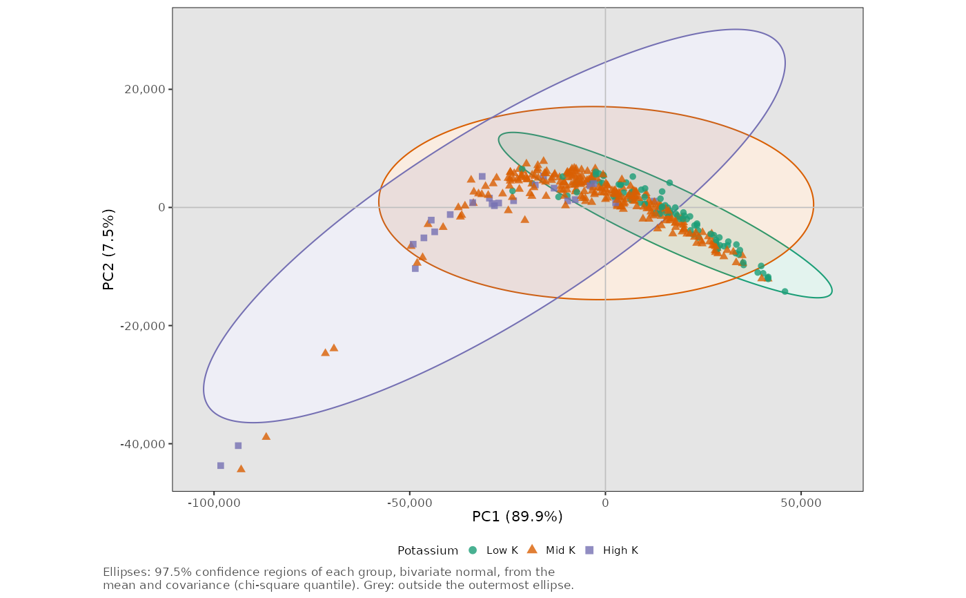
With ellipse = TRUE, a confidence ellipse is drawn for each group of a discrete colour (or for all the samples otherwise), with ConfidenceEllipse::confidence_ellipse(), at each level of conf_level (0.975 by default). It covers the region expected to hold that share of the samples of the group if they follow a bivariate normal distribution, from their mean and covariance, or from robust estimates (MCD) with robust = TRUE, which resist outlying samples. distribution = "hotelling" uses the quantile of Hotelling's \(T^2\) distribution, which accounts for the uncertainty of the estimates and suits small groups. Robust estimates need larger groups (the MCD fits a subset of about three quarters of the samples): with fewer than about 10 samples per group, their ellipses can be flat or leave out several samples. Groups with fewer than 4 samples get no ellipse.

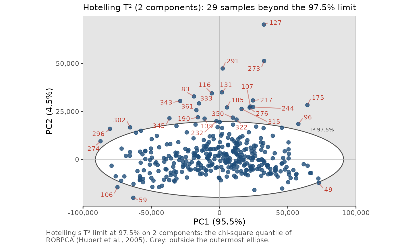
With hotelling = "all", the ellipses of Hotelling's \(T^2\) at each level of conf_level (97.5% by default) are drawn for all the samples, and the samples beyond the limit at the highest level of \(T^2\) on k components are counted in the subtitle, circled in red with flag = TRUE and labeled with label (each independently of the other): the classical outlier limits of a score plot. For a PCA model (stats::prcomp(), robpca(), rospca() or macropca()), \(T^2\) is that of the model: the scores divided by the variances of the components (the robust eigenvalues of a robust fit), so the ellipses are centered at 0 with the axes of the components, and semi-axes \(\sqrt{\lambda_a L}\) for the limit \(L\). The limit is the F (or Beta) limit of hotelling_t2() for a stats::prcomp() fit, and the chi-square quantile of ROBPCA for a robust fit, whose flagged samples are then the leverage points of plot_outlier_map() (with k its number of components and conf_level = 0.975). The scores of the outlying samples then do not inflate or tilt the ellipses. For other embeddings, \(T^2\) is computed from the mean and covariance of the samples (with hotelling_t2() and HotellingEllipse::ellipseCoord()). With hotelling = "group", each group of a discrete colour gets its own ellipses and limits, from its mean and covariance, which flags the samples atypical of their own group. The ellipses are labeled with their level (instead of a legend), and drawn for the two components shown, while the limits use k components, so with k > 2 a flagged sample can lie inside the ellipses. With ellipse = TRUE, the confidence ellipses are always computed from the samples shown. Without groups, ellipse = TRUE and hotelling = "all" would draw two ellipses of all the samples: only the \(T^2\) ellipse is drawn, with a warning. With groups, both are drawn: the confidence ellipses of the groups and the \(T^2\) limits of all the samples. \(T^2\) suits linear scores such as PCA or PLS; on a UMAP map, whose distances are not meaningful, prefer ellipse.

Style. The panel is grey outside the outermost ellipse (of \(T^2\), or of each group) and white inside, so that the samples beyond the limits stand out (panel = "white" for a white panel), with no grid and a fixed aspect_ratio (0.7 by default; NULL lets the plot fill the space, "equal" gives both axes the same scale), and thin light grey lines through the origin (when it lies in the range of the samples, as for centered scores). Without ellipses, the panel is white. The groups of a discrete colour also get their own point shapes (shapes), and the axes plain numbers. A caption says what the ellipses and limits are (their level, distribution and estimates), which readers cannot tell from the plot.

Publication figures. Make the plot at its printed size, with base_size set to the text size of the journal, for example ggsave("scores.pdf", p, width = 85, height = 75, units = "mm") with base_size = 8 for a single column.

Axes. For a stats::prcomp() fit or a robust PCA, the axis titles give the share of the variance of each component: of the total variance for stats::prcomp(), and of the variance of the k components of the model for robpca(), rospca() and macropca(), which estimate only these. With groups, the ellipses (confidence, or \(T^2\) with hotelling = "group") are filled with the color of their group.

Point size. size is a number, or a numeric variable (a column of data or a vector with one value per sample), such as the concentration of an element, which sets the size of each point, with a legend.

Biplot. With biplot = TRUE (for a stats::prcomp() fit or a robust PCA), the loadings of the two components are drawn over the scores: all the variables as faint points, and the biplot_top longest as labeled arrows. For spectra, the arrows are the local peaks of the loading length along the wavelength, one per emission line, labeled with their wavelength. Each axis of loadings is scaled to the range of its scores, and read on the top and right axes. A sample lies toward the arrows of the variables in which it is high.

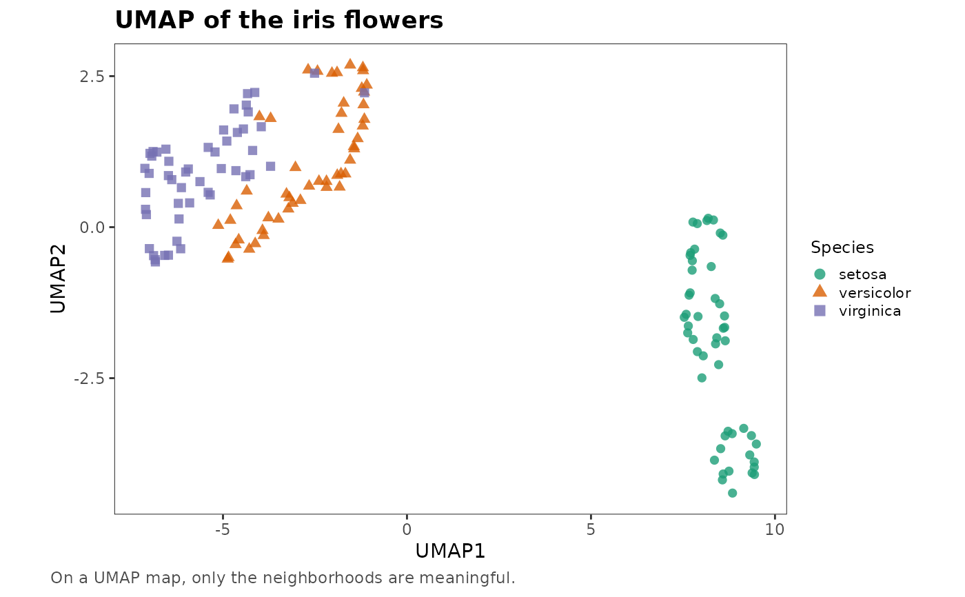
In a UMAP embedding, only the neighborhoods are meaningful: the sizes of the clusters and the distances between them are not, and they change with neighbors and min_dist. Read the plot as a map of which samples are similar, not as a quantitative projection. When both axes are UMAP coordinates (named UMAP1, UMAP2, ..., as by embed::step_umap()), the lines through the origin are left out, and hotelling ("all" or "group") is ignored, with a warning: its \(T^2\) limits assume linear scores.

Author

Christian L. Goueguel

Examples

# robust PCA of the forage spectra, with the Hotelling's T-squared limit
if (rlang::is_installed("HotellingEllipse", version = "1.3.0")) {
  data(forageLIBS)
  # the 380-430 nm window (Ca II H and K lines)
  wl <- suppressWarnings(as.numeric(names(forageLIBS)))
  set.seed(1)
  forageLIBS[which(wl > 380 & wl < 430)] |>
    center() |>
    robpca(k = 2) |>
    plot_embedding(hotelling = "all", flag = FALSE, label = TRUE)
}


# PCA of the K I lines, the samples grouped by potassium level, for a
# journal column
if (rlang::is_installed("ConfidenceEllipse")) {
  data(forageLIBS)
  wl <- suppressWarnings(as.numeric(names(forageLIBS)))
  pca <- stats::prcomp(forageLIBS[which(wl > 760 & wl < 772)])
  level <- cut(forageLIBS$K, 3, labels = c("Low K", "Mid K", "High K"))
  p <- plot_embedding(pca, colour = level, ellipse = TRUE, legend_title = "Potassium",
                      legend = "bottom", base_size = 8)
  p
  # ggplot2::ggsave("scores.pdf", p, width = 85, height = 80, units = "mm")
}
#> Warning: RGL: unable to open X11 display
#> Warning: 'rgl.init' failed, will use the null device.
#> See '?rgl.useNULL' for ways to avoid this warning.


# \donttest{
# UMAP map of the iris flowers, from embed::step_umap(): no lines through
# the origin, whose position means nothing on such a map
if (rlang::is_installed(c("recipes", "embed"))) {
  set.seed(1)
  umap <- recipes::recipe(Species ~ ., data = iris) |>
    recipes::step_normalize(recipes::all_predictors()) |>
    embed::step_umap(recipes::all_predictors(), neighbors = 15) |>
    recipes::prep() |>
    recipes::bake(new_data = NULL)
  plot_embedding(umap, colour = Species, title = "UMAP of the iris flowers")
}

# }