Robust PCA by Casewise and Cellwise Weighting (cellPCA)

Robust PCA that handles outlying observations (casewise outliers), outlying cells (cellwise outliers) and missing values by minimizing a single objective function: the cellPCA method of Centofanti, Hubert and Rousseeuw. Each cell and each observation gets a weight between 0 and 1 that reflects its outlyingness, and regular cells and observations are not downweighted, which makes cellPCA more efficient than macropca(). The iterations are computed in C++. The results have the same form as those of robpca(), so that predict(), plot_outlier_map() and plot_cell_map() work the same way.

Usage

cellpca(
  x,
  k = NULL,
  alpha = 0.5,
  kmax = 10,
  var_explained = 0.8,
  scale = FALSE,
  ndir = 250,
  maxiter = 1000,
  tol = 1e-06,
  max_col_frac = 0.5,
  od_cutoff = c("simulated", "chisq")
)

Arguments

x: A numeric matrix or data frame, with one observation per row. Missing values are allowed.
k: The number of principal components. If NULL (default), it is chosen from var_explained and kmax.
alpha: The robustness parameter, between 0.5 and 1: the fraction of observations used in the fit. Default is 0.5.
kmax: The maximum number of components. Default is 10.
var_explained: The fraction of variance used to choose k when it is not given. Default is 0.8.
scale: A logical: scale the variables by their robust scale (FALSE, default: they are only centered, so that intense emission lines are not outweighed by noise and continuum channels).
ndir: The number of random directions of the outlyingness, or "all". Default is 250.
maxiter, tol: The maximum number of iterations, and the tolerance on the relative change of the fit. Defaults are 1000 and 1e-6.
max_col_frac: The largest fraction of cells of a variable that can get a zero weight. Default is 0.5.
od_cutoff: How to compute the cut-off of od: "simulated" (default) or "chisq". See Details.

Value

An object of class specproc_cellpca (inheriting from specproc_robpca), with the components described in robpca() and macropca(), and:

cell_weights: the cellwise weights (0 for missing cells).
case_weights: the casewise weights.
deviation: the standardized casewise total deviations.
fitted: the fitted values $\hat{X}$.
imputed: the data in which the outlying cells are moved toward the fit in proportion to their weights, and the missing cells are replaced by the fit, so that the projection of each observation on the subspace is its fitted value.
sigma1, sigma2: the scales of the cellwise residuals and of the casewise total deviations; resid_scale: the scales of the final residuals.
objective: the objective at each iteration; iterations and converged.

Details

cellPCA approximates the data by a fit $\hat{X} = 1_n \mu^T + U V^T$ of rank k that minimizes $$\hat\sigma_2^2 \frac{1}{n} \sum_{i=1}^n m_i \rho_2\left(\frac{t_i}{\hat\sigma_2}\right), \quad t_i = \sqrt{\frac{1}{m_i} \sum_{j=1}^p m_{ij} \hat\sigma_{1,j}^2 \rho_1\left(\frac{x_{ij} - \hat{x}_{ij}}{\hat\sigma_{1,j}}\right)}$$ where $m_{ij}$ is 0 for a missing cell and 1 otherwise and $m_i$ is the number of observed cells of observation $i$. The bounded function $\rho_1$ limits the effect of the outlying cells (the residuals of variable $j$ divided by their scale $\hat\sigma_{1,j}$), and $\rho_2$ that of the outlying observations (the casewise total deviations $t_i$ divided by their scale $\hat\sigma_2$). Both are hyperbolic tangent functions (Hampel et al., 1981): $\rho_1$ with $b = 1.5$ and $c = 4$, and $\rho_2$ with $b$ and $c$ the 0.70 and 0.99 quantiles of the standardized total deviations of simulated Gaussian residuals. Their weights $\psi(z)/z$ are 1 in the central region and 0 beyond $c$.

The algorithm follows the reference code of the authors:

Initial fit. A macropca() fit (with alpha, kmax, var_explained, scale and ndir), which also chooses k when it is NULL, with its scores computed from the data whose flagged and missing cells are imputed by the fit.
Scales. $\hat\sigma_{1,j}$ is the M-scale of the residuals of variable $j$, and $\hat\sigma_2$ that of the total deviations (with $\rho_{1.5,4}$: 50% breakdown, consistent at the normal distribution). They are kept fixed.
Iteratively reweighted least squares. The loadings (one variable at a time, with the casewise and cellwise weights) and the scores (one observation at a time, with the cellwise weights) are updated by weighted least squares, the loadings are orthonormalized, the center is updated, and so are the weights, until the fit $U V^T$ changes by less than tol (relative), at most maxiter times. Each iteration decreases the objective. If more than max_col_frac of the cells of a variable get a zero weight, the previous iteration is kept.
Principal directions. The center and the eigenvectors within the subspace are estimated by the deterministic MCD of the scores of the observations with a non-zero casewise weight (the exact MCD when k = 1), and the sign of each loading vector is set so that its largest element is positive.

The residuals of each variable are then standardized by their M-scale, and the cells beyond $\sqrt{\chi^2_{1, 0.99}}$ are flagged. As in the enhanced outlier map of the paper, od is the norm of the standardized residuals of each observation, and sd the score distance of its projection on the subspace (of its robust scores when it has missing cells). The cut-off of sd is $\sqrt{\chi^2_{k, 0.99}}$. That of od is, by default (od_cutoff = "simulated"), the 0.99 quantile of the od of a cellPCA fit to clean data simulated from the fit, as in the reference code (this needs a second fit); "chisq" uses $\sqrt{\chi^2_{p, 0.99}}$ instead.

New observations, with missing or outlying cells, are projected by the robust regression of their observed cells on the loadings, also in C++.

References

Centofanti, F., Hubert, M., Rousseeuw, P.J. (2026). Robust principal components by casewise and cellwise weighting. Technometrics. doi:10.1080/00401706.2026.2643216
Hampel, F.R., Rousseeuw, P.J., Ronchetti, E. (1981). The change-of- variance curve and optimal redescending M-estimators. Journal of the American Statistical Association, 76(375):643-648.
Hubert, M., Rousseeuw, P.J., Van den Bossche, W. (2019). MacroPCA: an all-in-one PCA method allowing for missing values as well as cellwise and rowwise outliers. Technometrics, 61(4):459-473.

Author

Christian L. Goueguel

Examples

data(forageLIBS)
# the K I resonance lines
wl <- suppressWarnings(as.numeric(names(forageLIBS)))
spectra <- forageLIBS[which(wl > 760 & wl < 780)]
set.seed(1)
fit <- cellpca(spectra, k = 2, od_cutoff = "chisq")
fit
#> Robust PCA by casewise and cellwise weighting (cellPCA)
#> 
#> Observations:   368 (h = 185)
#> Variables:      245
#> Components:     2
#> Eigenvalues:    322134967  14963319
#> Flagged cells:  4052
#> Downweighted observations: 140
#> IRLS iterations: 98
#> 
#> Outlier types:
#> 
#>            regular      good leverage orthogonal outlier       bad leverage 
#>                255                  1                 90                 22 
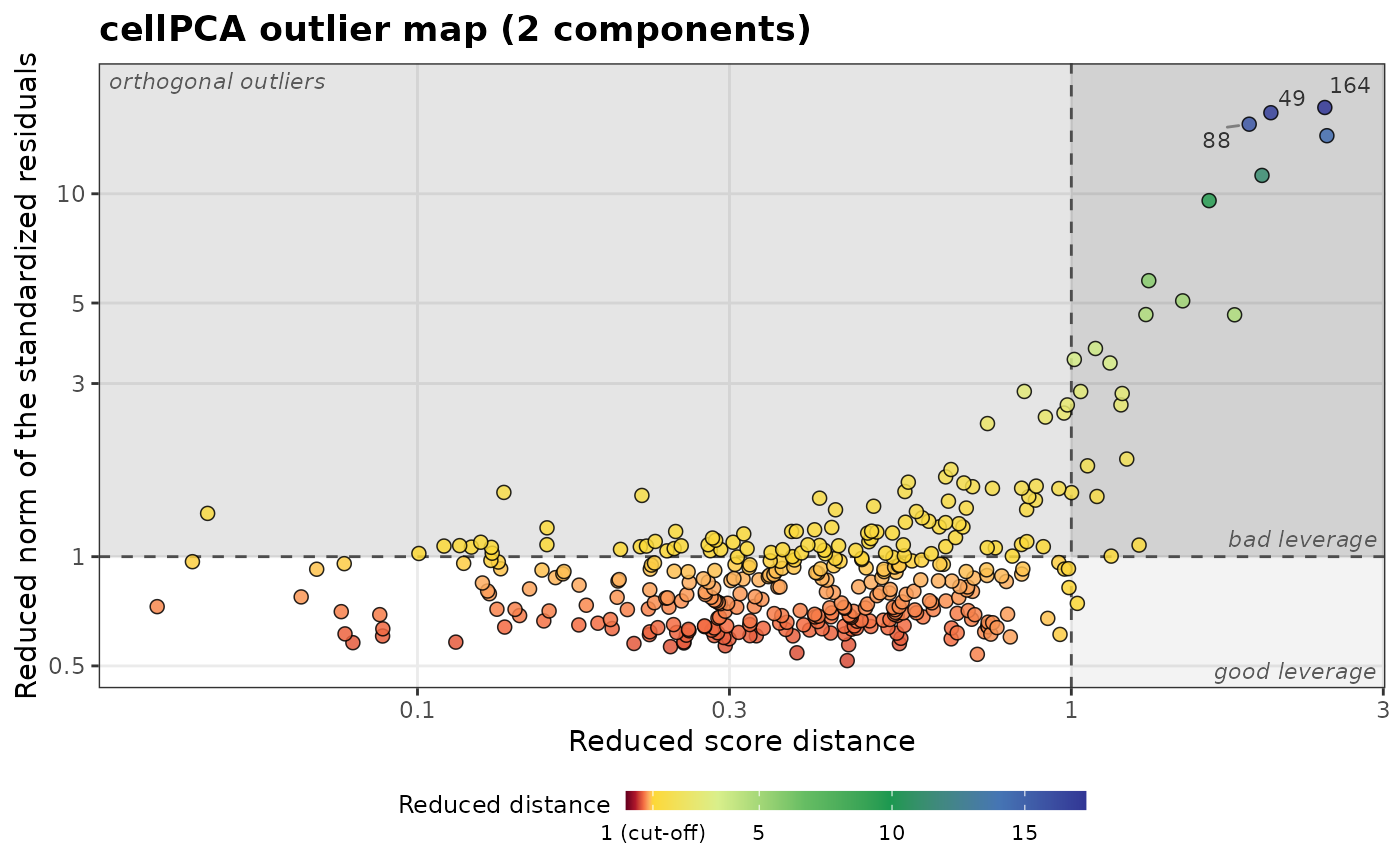
plot_outlier_map(fit, shade = TRUE, relative = TRUE, log = TRUE, colour_by = "distance")

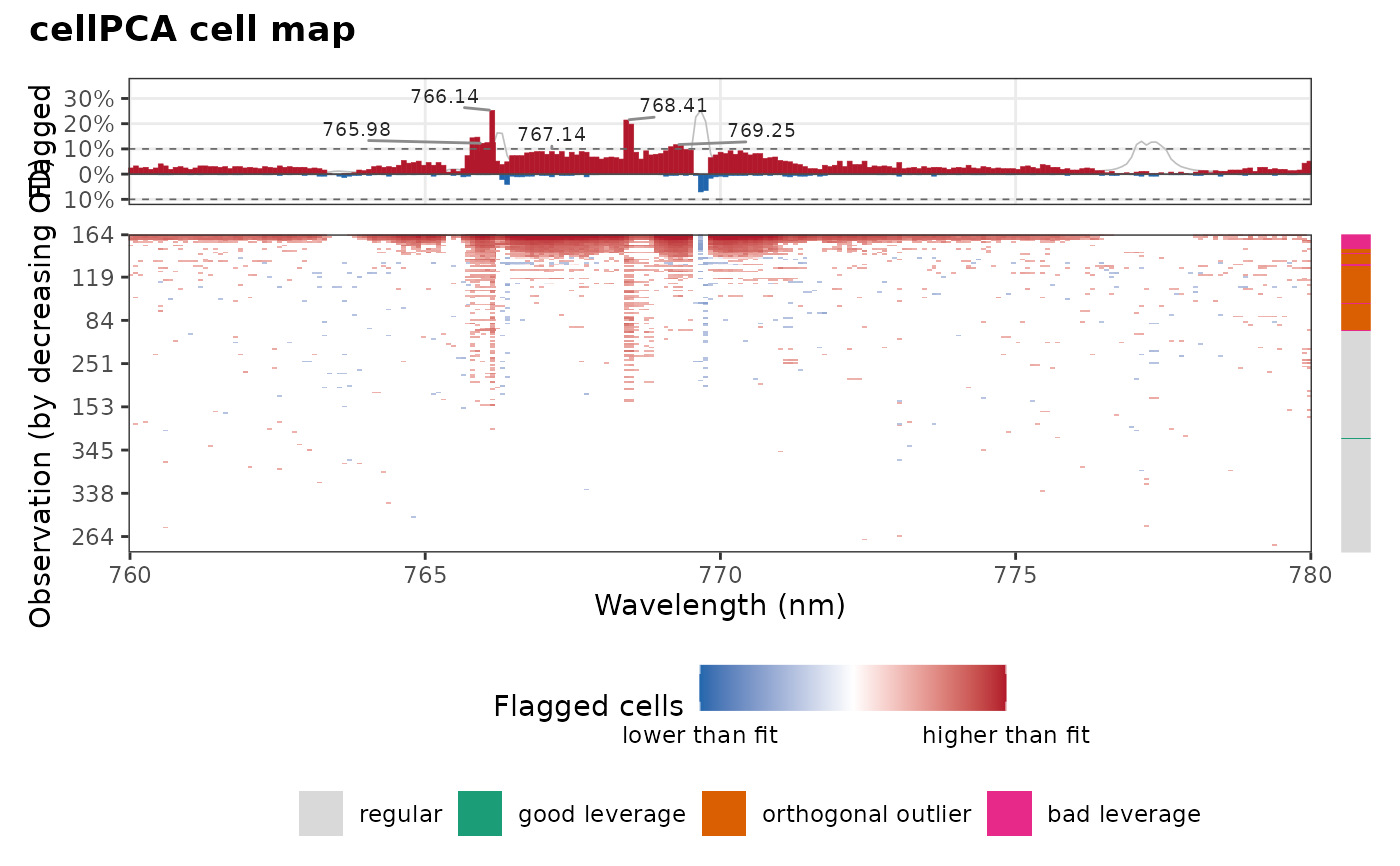
plot_cell_map(fit, order = "od")