
This function performs baseline correction on the spectral matrix by estimating and removing the continuous background emission using least-squares polynomial curve fitting approach.
Usage
baseline_lsp(
  x,
  degree = 4,
  tol = 0.001,
  max.iter = 100,
  method = c("imodpoly", "modpoly")
)
Arguments
- x
A matrix or data frame, with one spectrum per row.
- degree
An integer specifying the degree of the polynomial fitting function. The default value is 4.
- tol
A numeric value representing the tolerance for the difference between iterations. The default value is 1e-3.
- max.iter
An integer specifying the maximum number of iterations for the algorithm. The default value is 100.
- method
The algorithm:
"imodpoly"(default) or"modpoly". See Details.
Value
A list with two elements:
correction: The baseline-corrected spectral matrix.background: The fitted background emission.
Details
Two iterative polynomial fits are available:
"modpoly": the modified polynomial fit of Lieber and Mahadevan-Jansen (2003). A polynomial is fitted to the spectrum, the points of the spectrum above the fit are replaced by the fit, and the fit is repeated, so that the peaks are progressively removed. The first fits are pulled up by strong peaks, and the ends of the spectrum, where nothing pulls the polynomial back, can then fall far below the background."imodpoly"(default): the improved modified polynomial fit of Zhao et al. (2007). The points more than one standard deviation of the residuals above the first fit (the peaks) are left out of the following fits, and the remaining points are clipped at the fit plus the standard deviation of the residuals, rather than at the fit. The iterations stop when this standard deviation changes by less thantol(relative). The baseline follows the background up to the ends of the spectrum and passes through its noise.
References
Lieber, C.A., Mahadevan-Jansen, A., (2003). Automated method for subtraction of fluorescence from biological Raman spectra. Applied Spectroscopy, 57(11):1363-1367
Zhao, J., Lui, H., McLean, D.I., Zeng, H., (2007). Automated autofluorescence background subtraction algorithm for biomedical Raman spectroscopy. Applied Spectroscopy, 61(11):1225-1232.
Examples
data(forageLIBS)
spectrum <- forageLIBS[1, -(1:14)]
wl <- as.numeric(names(spectrum))
in_region <- wl > 240 & wl < 300
region <- spectrum[in_region]
res <- baseline_lsp(region, degree = 4)
oldpar <- par(mfrow = c(2, 1), mar = c(4, 4, 2, 1))
# the spectrum and its fitted baseline
plot(wl[in_region], unlist(region), type = "l", col = "grey40", ylim = c(800, 3000),
xlab = "Wavelength (nm)", ylab = "Counts", main = "Spectrum and baseline")
lines(wl[in_region], unlist(res$background), col = "red")
# the corrected spectrum: the background is now around zero
plot(wl[in_region], unlist(res$correction), type = "l", col = "grey40",
ylim = c(-200, 2000), xlab = "Wavelength (nm)", ylab = "Counts",
main = "Corrected spectrum")
abline(h = 0, col = "red", lty = 2)
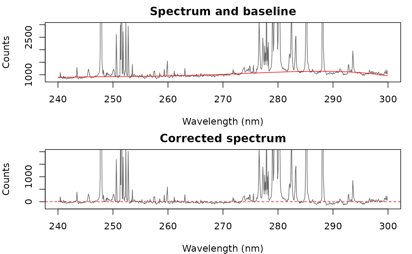 par(oldpar)