
Baseline correction based on asymmetric least squares (ALS) algorithm as proposed by Eilers et al. (2005).
Arguments
- x
A numeric matrix or data frame, with one spectrum per row.
- lambda
A numeric value specifying the smoothing parameter, which controls the amount of curvature allowed for the baseline. The smaller the lambda, the more curvature in the baseline fitting. Default is 1000.
- p
A numeric value specifying the extent of asymmetry required of the fit. Larger values allow more negative-going regions. Smaller values disallow negative-going regions.
pmust be between 0 and 1. Default is 0.001.- max.iter
Maximum number of iterations for the algorithm. Default is 10.
Value
A list containing two tibbles:
correction: The baseline-corrected spectral matrix.background: The fitted background emission.
Details
The function applies Eilers' method based on a Whittaker filter. The algorithm estimates a baseline curve by minimizing the asymmetric least squares criterion, which allows for different weights for positive and negative residuals. The resulting baseline curve is subtracted from the input data, providing a baseline-corrected version.
The penalized system is pentadiagonal and is solved in C++ with a banded Cholesky decomposition, so the cost grows linearly with the number of spectral channels. Negative values in the corrected spectra are kept as they are (they typically reflect noise around the baseline).
References
Eilers, P.H.C., Boelens, H.F.M., (2005). Baseline correction with asymmetric least squares smoothing. Leiden University Medical Centre report.
Examples
data(forageLIBS)
spectrum <- forageLIBS[1, -(1:14)]
wl <- as.numeric(names(spectrum))
in_region <- wl > 240 & wl < 300
region <- spectrum[in_region]
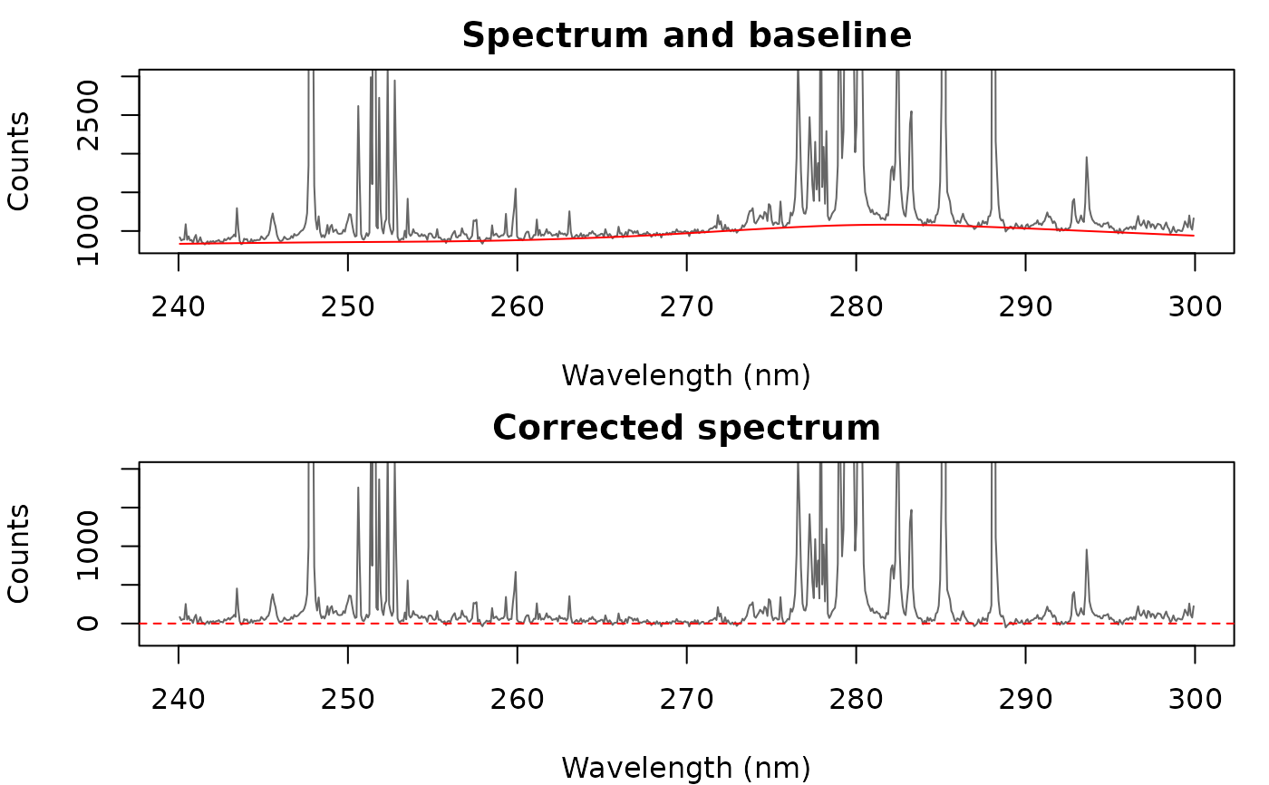
res <- baseline_als(region, lambda = 1e6)
oldpar <- par(mfrow = c(2, 1), mar = c(4, 4, 2, 1))
# the spectrum and its fitted baseline
plot(wl[in_region], unlist(region), type = "l", col = "grey40", ylim = c(800, 3000),
xlab = "Wavelength (nm)", ylab = "Counts", main = "Spectrum and baseline")
lines(wl[in_region], unlist(res$background), col = "red")
# the corrected spectrum: the background is now around zero
plot(wl[in_region], unlist(res$correction), type = "l", col = "grey40",
ylim = c(-200, 2000), xlab = "Wavelength (nm)", ylab = "Counts",
main = "Corrected spectrum")
abline(h = 0, col = "red", lty = 2)
 par(oldpar)