ssh = suppressPackageStartupMessagesChemometric Modeling with Tidymodels: A Tutorial for Spectroscopic Data
R
Tidymodels
Chemometrics
Machine Learning
Spectroscopy
In this post, we demonstrate how to build robust chemometric models for spectroscopic data using the Tidymodels framework in R. This workflow is designed to cater to beginners and advanced practitioners alike, offering an end-to-end guide from data preprocessing to model evaluation and interpretation.

For this tutorial, we use the beer dataset, publicly available and commonly used for spectroscopy-based regression problems. This dataset contains near-infrared spectroscopy (NIRS) data of beer samples alongside measurements of the original gravity (alcoholic beverage), which serves as the target variable. Original gravity (OG) is one of the primary metrics used by brewers to estimate the potential alcohol content of the beer, as it reflects the fermentable sugar content available for yeast metabolism. By analyzing OG alongside the NIRS spectra, we can explore how the spectral data correlates with this fundamental brewing property, offering insights into the chemical composition and quality of the beer samples.
Setup
Below, we use suppressPackageStartupMessages to suppress startup messages for clarity and load essential packages.
tidyversefor data manipulation and visualization.tidymodelsfor modeling workflows and machine learning.tidymodels_prefer()ensures consistency across conflicting tidymodels functions.
ssh(library(tidyverse))
ssh(library(tidymodels))
tidymodels_prefer()Additional libraries include:
kknn: Implements k-nearest neighbors (KNN).glmnet: Used for elastic net regression.ranger: Used for random forest.plsmod: Supports partial least squares (PLS) regression.magrittr: Provides pipe operators (%>%, %<>%).patchwork: Simplifies combiningggplot2plots.
library(kknn)
library(plsmod)
ssh(library(glmnet))
ssh(library(ranger))ssh(library(magrittr))
library(patchwork)We set a custom theme with a clean white background and adjusted sizes for all ggplot2 plots.
base_size = 15
theme_bw(
base_size = base_size,
base_line_size = base_size / 22,
base_rect_size = base_size / 15
) %>%
theme_set()Dataset Overview
We begin by loading the beer dataset and identifying the spectral predictor columns, which correspond to the NIRS wavelength variables. Usually, I prefer storing spectral wavelengths as character strings in a variable named wavelength because it makes data manipulation easier. This approach enhances flexibility when selecting, filtering, or grouping columns, simplifies integration with tidyverse functions, and ensures compatibility with tidymodels preprocessing workflows.
beer_data <- read_csv("beer.csv", show_col_types = FALSE)
wavelength <- beer_data %>% select(starts_with("xtrain")) %>% names()Previewing the first rows of the dataset helps us ensure its integrity and understand its structure.
beer_data %>% head(5) %>% DT::datatable()Show the code
p <- beer_data %>% mutate(spectra_id = paste0("s", 1:80)) %>%
pivot_longer(
cols = -c(originalGravity, spectra_id),
names_to = "wavelength",
values_to = "intensity"
) %>%
mutate(wavelength = rep(seq(1100, 2250, 2), times = 80)) %>%
ggplot() +
aes(x = wavelength, y = intensity, colour = originalGravity, group = spectra_id) +
geom_line() +
scale_color_viridis_c(option = "inferno", direction = 1) +
labs(
x = "Wavelength [nm]",
y = "Absorbance [arb. units]",
title = "NIRS Spectra of Beer Samples",
subtitle = "Contains 80 samples, measured from 1100 to 2250 nm",
color = "Original Gravity") +
theme_minimal()
plotly::ggplotly(p)Supervised Learning Techniques
For this analysis, we’ll evaluate and compare the performance of four supervised learning algorithms, categorized by their linearity or modeling approach (parametric vs. non-parametric):
| Algorithm | Acronym | Approach |
|---|---|---|
| sparse Partial Least Squares | sPLS |
Linear |
| Elastic Net | ENet |
Linear |
| k-Nearest Neighbors | KNN |
Non-linear |
| Random Forests | RF |
Non-linear |
Step 1: Data Splitting
To ensure unbiased model evaluation, we partition the data into training (80%) and testing (20%) sets, employing stratified sampling based on the target variable’s distribution.
set.seed(123)
split_data <- initial_split(beer_data, prop = 0.8, strata = originalGravity)
train_data <- training(split_data)
test_data <- testing(split_data)Step 2: Cross-Validation
We use a 5-fold repeated cross-validation strategy for hyperparameters tuning and performance evaluation, minimizing the risk of overfitting.
cv_folds <- vfold_cv(train_data, v = 5, repeats = 3)Interestingly, the vfold_cv function provides a powerful way to visualize the distribution of data across folds, allowing us to confirm that the stratification and splits are evenly balanced. This ensures that each fold accurately represents the overall dataset, enhancing the reliability of cross-validation results.
Show the code
cv_folds %>%
tidy() %>%
ggplot(aes(x = Fold, y = Row, fill = Data)) +
geom_tile() +
facet_wrap(~Repeat) +
scale_fill_brewer(palette = "Paired")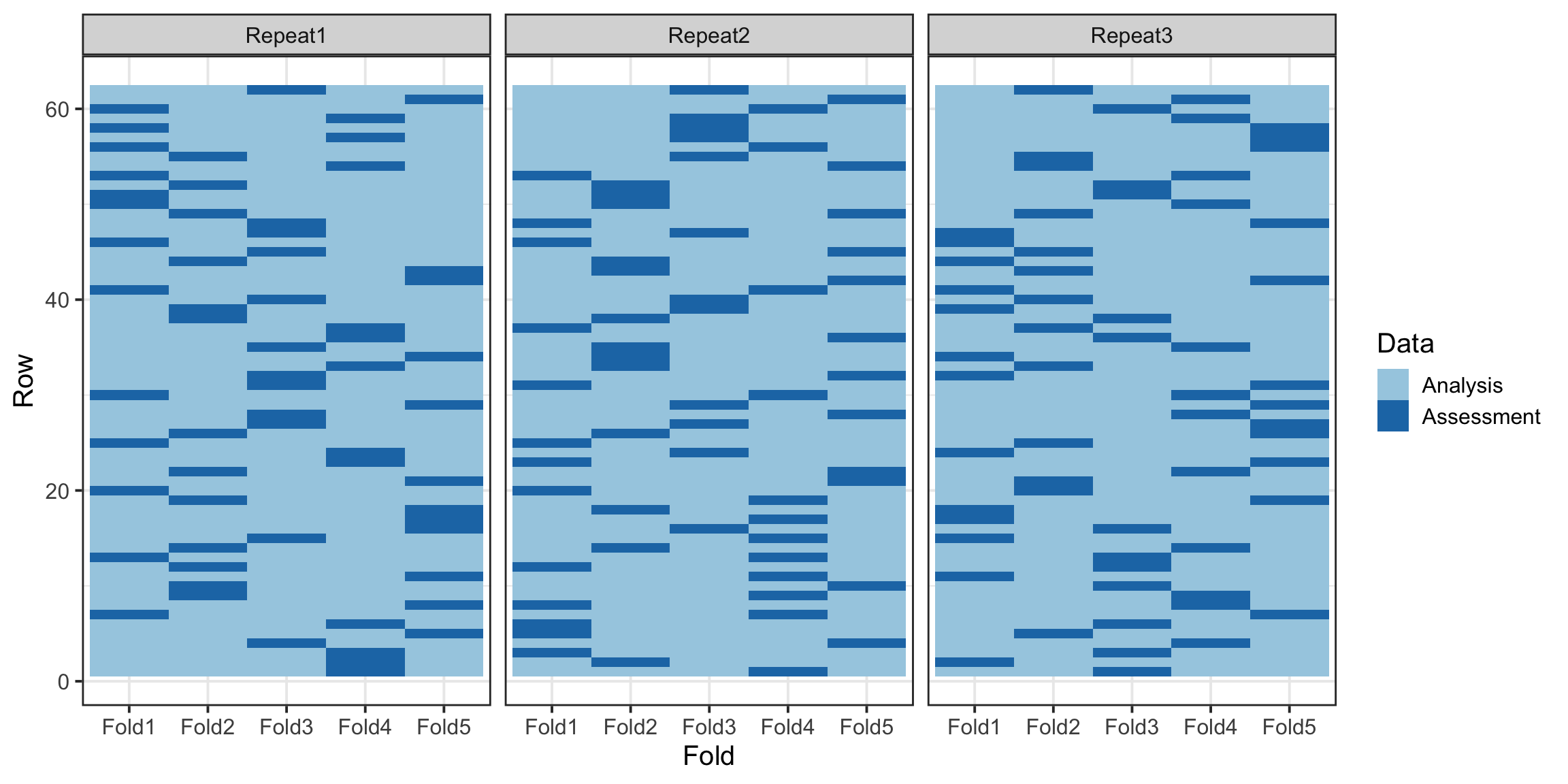
Step 3: Preprocessing
Preprocessing spectral data is a vast and intricate topic, deserving its own dedicated discussion, which we will explore in a future post. For this tutorial, we remove zero-variance predictors, and center the spectra intensity to ensure the data is well-suited for modeling.
tidymodels provides a wide array of preprocessing steps through its versatile step_* functions. These functions allow for comprehensive data transformations, including centering, scaling, feature selection, and more, to be seamlessly integrated into the modeling workflow. Additionally, tidymodels offers the flexibility to create custom recipe steps, enabling you to design and implement tailored data transformations that meet your specific needs.
base_recipe <- recipe(originalGravity ~ ., data = train_data) %>%
update_role(originalGravity, new_role = "outcome") %>%
update_role(all_of(wavelength), new_role = "predictor") %>%
step_zv(all_predictors()) %>%
step_center(all_predictors())For comparison with the base preprocessing step, we introduce an additional step that applies Principal Component Analysis (PCA) to the predictor variables. This transformation reduces the dimensionality of the data while retaining the most significant variance.
pca_recipe <- base_recipe %>%
step_pca(all_predictors())Step 4: Model Specifications
We now define model specifications for each algorithm, incorporating hyperparameter tuning within the tidymodels framework. Notably, the tune function is used to specify hyperparameters that require optimization during the tuning process. For parameters with predefined values, these can be directly assigned within their allowable range.
# k-Nearest Neighbors (KNN)
knn_spec <- nearest_neighbor() %>%
set_args(neighbors = tune(), weight_func = tune(), dist_power = tune()) %>%
set_engine('kknn') %>%
set_mode('regression')
# Partial Least Squares Regression (PLSR)
spls_spec <- pls() %>%
set_args(predictor_prop = tune(), num_comp = tune()) %>%
set_engine('mixOmics') %>%
set_mode('regression')
# Elastic Net (ENet)
enet_spec <-linear_reg() %>%
set_args(penalty = tune(), mixture = tune()) %>%
set_engine("glmnet") %>%
set_mode("regression")
# Random Forest (RF)
rf_spec <- rand_forest() %>%
set_args(mtry = tune(), trees = tune(), min_n = tune()) %>%
set_engine("ranger") %>%
set_mode("regression")Step 5: Model Training and Tuning
Using the workflow_set function, we define a workflow for each model and tune hyperparameters using a grid search, and enable parallel processing using 4 CPU cores, accelerating computation during tuning.
wflowSet <- workflow_set(
preproc = list(base = base_recipe, pca = pca_recipe),
models = list(
knn = knn_spec,
spls = spls_spec,
enet = enet_spec,
rf = rf_spec),
cross = TRUE
)As mentionned earlier, we opted to train each model using both the base preprocessing approach and the PCA-transformed data. This strategy results in a total of eight unique training models as follows:
wflowSet# A workflow set/tibble: 8 × 4
wflow_id info option result
<chr> <list> <list> <list>
1 base_knn <tibble [1 × 4]> <opts[0]> <list [0]>
2 base_spls <tibble [1 × 4]> <opts[0]> <list [0]>
3 base_enet <tibble [1 × 4]> <opts[0]> <list [0]>
4 base_rf <tibble [1 × 4]> <opts[0]> <list [0]>
5 pca_knn <tibble [1 × 4]> <opts[0]> <list [0]>
6 pca_spls <tibble [1 × 4]> <opts[0]> <list [0]>
7 pca_enet <tibble [1 × 4]> <opts[0]> <list [0]>
8 pca_rf <tibble [1 × 4]> <opts[0]> <list [0]>ctrl_grid <- control_grid(
verbose = TRUE,
allow_par = TRUE,
extract = NULL,
save_pred = TRUE,
pkgs = c("doParallel", "doFuture"),
save_workflow = FALSE,
event_level = "first",
parallel_over = "resamples"
)cl <- parallel::makePSOCKcluster(4)
doParallel::registerDoParallel(cl)wflowSet %<>%
workflow_map(
fn = "tune_grid",
resamples = cv_folds,
grid = 10,
metrics = metric_set(rmse, mae, rsq),
control = ctrl_grid,
seed = 3L,
verbose = TRUE
)parallel::stopCluster(cl)Next, we utilize the rank_results function to systematically rank the training models based on key performance metrics such as the root mean squared error (RMSE), the mean absolute error (MAE), and the coefficient of determination \((R^2)\). Following this, we visualize the model performance with error bars, providing a clear and insightful comparison of their predictive capabilities.
wflowSet %>%
rank_results(rank_metric = "rmse") %>%
relocate(c(rank, model, .metric, mean, std_err), .before = wflow_id) %>%
mutate(mean = round(mean, 4), std_err = round(std_err, 4)) %>%
DT::datatable(rownames = FALSE, filter ="top")wflowSet %>% autoplot(std_errs = qnorm(0.95), type = "wflow_id") +
ggsci::scale_color_lancet() +
theme(legend.position = "bottom") +
ylab("")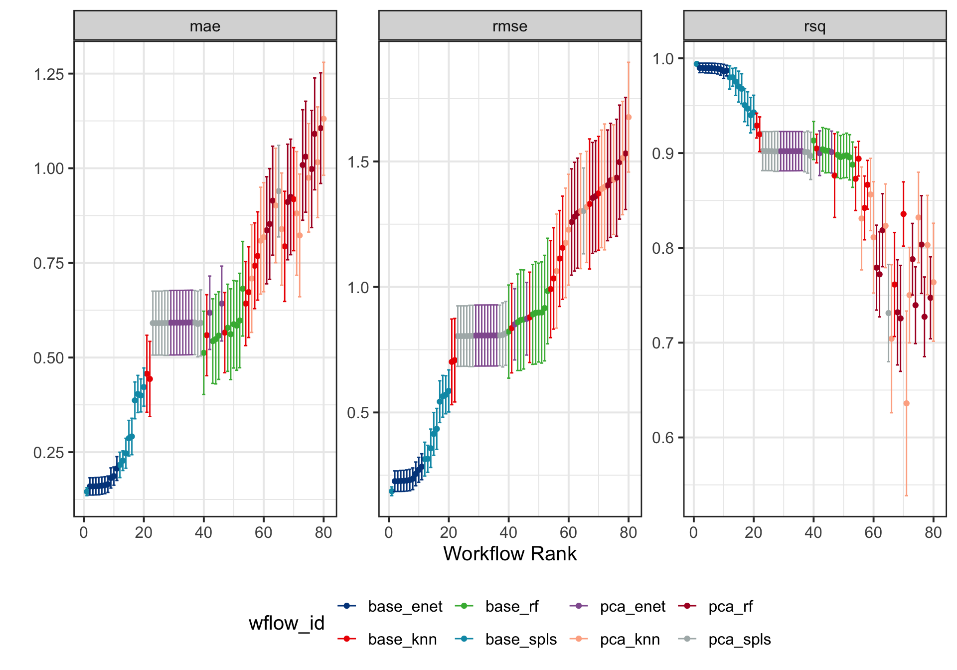
Step 6: Model Selection
By configuring the autoplot function with the argument select_best = TRUE, we rank the training models while visually emphasizing the best-performing model, making it easy to identify the optimal choice for further evaluation.
wflowSet %>% autoplot(select_best = TRUE, std_errs = qnorm(0.95), type = "wflow_id") +
geom_point(size = 3) +
ggsci::scale_color_lancet() +
theme(legend.position = "bottom") +
ylab("")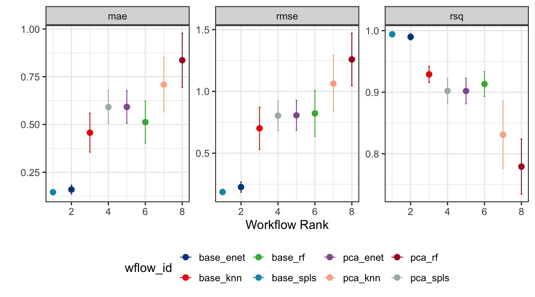
The extract_workflow_set_result function retrieves the optimized hyperparameter values for the best-performing model, as determined by the lowest RMSE. In this analysis, it determines the optimal settings for base_spls, specifically identifying the optimized number of latent variables (num_comp) and the proportion of predictors (predictor_prop) allowed to have non-zero coefficients.
best_model <- wflowSet %>%
extract_workflow_set_result("base_spls") %>%
select_best(metric = "rmse") %>%
print()# A tibble: 1 × 3
predictor_prop num_comp .config
<dbl> <int> <chr>
1 0.0633 3 Preprocessor1_Model01We use the collect_predictions function to gather the best-performing model’s training data and visualize the relationship between the actual and predicted values. This allows us to assess the model’s predictive accuracy. Additionally, we perform a residual analysis using standardized residuals to further evaluate the model’s performance and identify any potential areas for improvement.
train_results <- wflowSet %>%
collect_predictions() %>%
filter(wflow_id == "base_spls" & .config == best_model %>% pull(.config)) %>%
select(-.row)train_results %>%
mutate(
.pred = round(.pred, 2),
originalGravity = round(originalGravity, 4),
residuals = round((originalGravity - .pred)/sd((originalGravity - .pred)), 2)
) %>%
relocate(c(.pred, originalGravity, residuals, model), .before = wflow_id) %>%
DT::datatable(rownames = FALSE)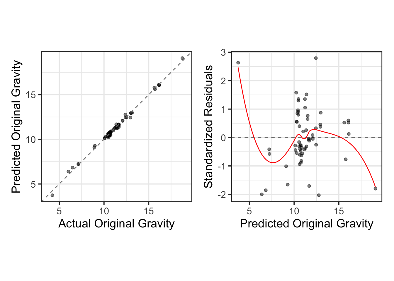
Step 7: Model Testing
Finally, we finalize the best-performing model (base_spls) by utilizing the extract_workflow and finalize_workflow functions. We then assess the model’s performance on the test set using last_fit(split = split_data), calculating key metrics to evaluate its accuracy. These metrics are retrieved using the collect_metrics() function.
As done previously, we visualize the results through actual vs. predicted plots, complemented by residual diagnostics, to provide a comprehensive evaluation of the model’s performance.
test_results <- wflowSet %>%
extract_workflow("base_spls") %>%
finalize_workflow(best_model) %>%
last_fit(split = split_data)test_results$.predictions[[1]] %>%
mutate(
.pred = round(.pred, 2),
originalGravity = round(originalGravity, 4),
residuals = round((originalGravity - .pred)/sd((originalGravity - .pred)), 2)
) %>%
relocate(residuals, .before = .config) %>%
DT::datatable(rownames = FALSE, width = 400)test_results %>%
collect_metrics() %>%
mutate(.estimate = round(.estimate, 4)) %>%
DT::datatable(rownames = FALSE, width = 400)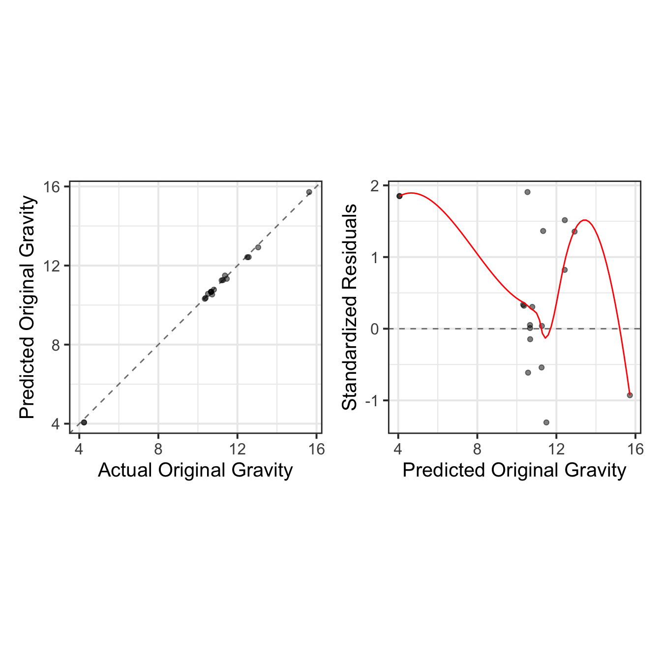
Conclusion
This tutorial showcased the versatility of the Tidymodels framework for chemometric applications. By leveraging its modular and tidy design, you can implement robust spectroscopic models tailored to your dataset, ensuring both accuracy and reproducibility.