Should We Use Standard Error or Standard Deviation?

One of the most common questions in statistics is whether to report standard error (SE) or standard deviation (SD) when presenting data. While these two measures are related, they serve fundamentally different purposes and choosing the wrong one can mislead your audience. Let’s break down when to use each.

Photo by Cody Board.

Standard Deviation: How spread out is your data?

Standard deviation (SD) tells us about the variability within our sample. It describes how spread out the individual data points are around the sample mean. Think of it as answering: “How much do individual observations typically differ from the average?”. SD is given by:

\[ \text{SD} = \frac{\sum^n_{i=1}(x_i-\bar{x})^2}{n-1} \]

Where, \(x_i\) ​is the individual data points, \(\bar{x}\) the sample mean, and \(n\) the sample size.

Notice the \(n−1\) in the denominator. This is called Bessel’s correction, and it adjusts for the fact that we’re estimating the population variance from a sample. Using \(n−1\) instead of \(n\) prevents underestimating variability. In essence:

Bessel’s correction compensates for the fact that a sample is typically less variable than the entire population. By using the sample mean, we’ve already “used up” one degree of freedom. It’s as if our effective sample size is reduced from \(n\) to \(n−1\). That’s why we often say that Bessel’s correction “adjusts the sample size.”

import numpy as np
import matplotlib.pyplot as plt

np.random.seed(42)
population = np.random.normal(loc=0, scale=1, size=1_000_000)
true_sd = np.std(population, ddof=0)
sample_sizes = np.logspace(1, 4, num=50, dtype=int)  # from 10 to 10,000

sd_n = []
sd_n1 = []

for n in sample_sizes:
    sample = np.random.choice(population, size=n, replace=False)
    sd_biased = np.sqrt(np.sum((sample - sample.mean())**2) / n)
    sd_unbiased = np.std(sample, ddof=1)
    sd_n.append(sd_biased)
    sd_n1.append(sd_unbiased)

plt.figure(figsize=(8,5))
plt.axhline(y=true_sd, color="black", linestyle="--", label="True population SD")
plt.plot(sample_sizes, sd_n, "r-", label="SD (divide by n)", markersize=5)
plt.plot(sample_sizes, sd_n1, "b-", label="SD (divide by n-1, Bessel)", markersize=5)
plt.xscale("log")
plt.xlabel("Sample size (n)")
plt.ylabel("Estimated SD")
plt.title("Effect of Bessel's Correction on SD Estimates")
plt.legend()
plt.grid(True, which="both", linestyle="--", alpha=0.6)
plt.show()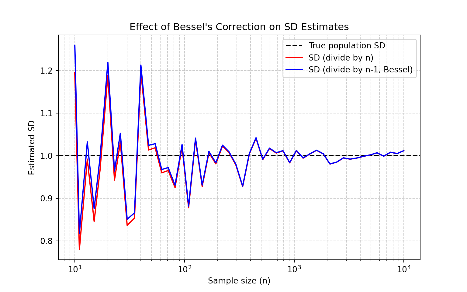

The figure above compares two ways of calculating the sample standard deviation across different sample sizes (\(n\) =10 to \(n\) =10,000). For small samples, the difference between dividing by \(n\) or \(n−1\) is large. Without Bessel’s correction, the population variability is underestimated. As the sample size increases, the bias shrinks and the two estimates converge.

In practice, we rarely have very large sample size. Using \(n−1\) ensures our standard deviation is an unbiased estimator of the population variability.

Standard Error: How precise is your mean?

Standard error tells us about the precision of our sample mean as an estimate of the population mean. It describes how much our sample mean would vary if we repeated the study many times. It answers:

“If we repeated this study many times, how much would the sample mean vary?”

Standard error is directly related to standard deviation:

\[ \text{SE} = \frac{\text{SD}}{\sqrt{n}} \]

Where \(n\) is the sample size. This relationship reveals something important: as your sample size increases, the standard error decreases (your estimate becomes more precise), but the standard deviation might stay roughly the same (the underlying variability in the population doesn’t change).

np.random.seed(123)
population = np.random.normal(loc=50, scale=10, size=1_000_000)
sample_sizes = [10, 20, 30, 40, 50, 60, 70, 80, 90, 100]

all_sample_means = []
all_sample_sizes = []

for n in sample_sizes:
    sample_means = [np.mean(np.random.choice(population, size=n, replace=False)) 
                    for _ in range(100)]
    all_sample_means.extend(sample_means)
    all_sample_sizes.extend([n] * 100)

all_sample_means = np.array(all_sample_means)
all_sample_sizes = np.array(all_sample_sizes)

plt.figure(figsize=(10, 8))

jitter = np.random.normal(0, 0.3, len(all_sample_sizes))
x_positions = all_sample_sizes + jitter
plt.scatter(x_positions, all_sample_means, alpha=0.6, s=20, color='black')

y_min, y_max = plt.ylim()
for y in range(int(y_min), int(y_max) + 1, 5):
    plt.axhline(y=y, color='gray', linestyle='-', alpha=0.3, linewidth=0.5)

population_mean = np.mean(population)
plt.axhline(y=population_mean, color='red', linestyle='--', alpha=0.7, linewidth=2)

plt.xlabel('Sample Size (n)', fontsize=15)
plt.ylabel('Sample Mean', fontsize=15)
plt.title('Distribution of Sample Means for Different Sample Sizes', fontsize=18)
plt.grid(True, alpha=0.3)
plt.xlim(5, 105);
plt.tight_layout()
plt.show()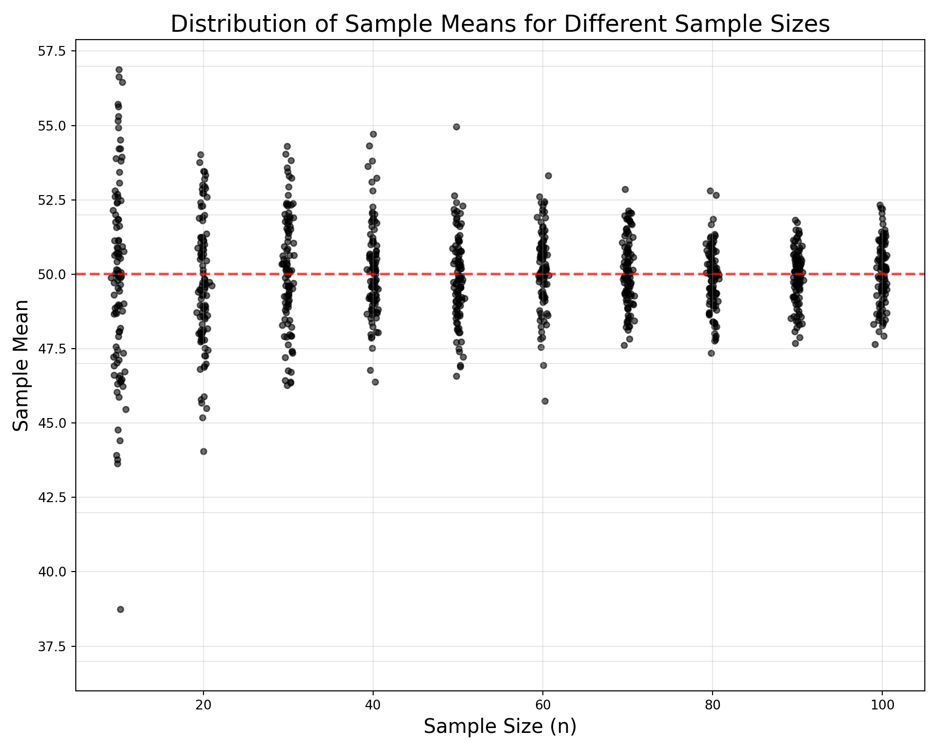

From the figure above, we observe several fundamental statistical principles in action. First, all distributions are precisely centered around the true population mean (indicated by the red dashed line), regardless of sample size. This demonstrates that sample means serve as unbiased estimators of the population parameter, a critical property ensuring our estimates are systematically accurate rather than consistently over- or under-estimating the true value.

More striking is the dramatic reduction in variability as we move from left to right across increasing sample sizes. The vertical spread of sample means becomes progressively tighter, providing compelling visual evidence that standard error decreases as sample size increases. This relationship follows the mathematical principle SE = σ/√n, meaning that precision improves predictably but at a diminishing rate, doubling the sample size reduces uncertainty by only √2, not by half. Perhaps most remarkably, each vertical column of points approximates a normal distribution, regardless of the original population’s shape. This illustrates the Central Limit Theorem in action: the sampling distribution of means becomes increasingly normal as sample size grows, even when sampling from non-normal populations. This powerful theorem provides the theoretical foundation for much of inferential statistics.

We use standard error when we want to communicate uncertainty about population parameters:

• Confidence intervals: SE helps calculate how precisely we’ve estimated the population mean
• Hypothesis testing: SE is crucial for determining statistical significance
• Comparing groups: When we want to know if observed differences likely reflect real population differences
• Meta-analyses: Combining results from multiple studies

Standard error is essential when making inferences beyond our sample to the broader population.

Summary

• Don’t use SE to make data look less variable: Some researchers inappropriately use standard error instead of standard deviation because SE is always smaller, making their data appear more consistent. This is misleading.
• Don’t use SD for inferential statistics: If you’re testing hypotheses or building confidence intervals, you need standard error, not standard deviation.
• Don’t confuse error bars: When creating graphs, be explicit about whether your error bars represent SD or SE. They tell completely different stories.